Main analysis
PGS calculation
We will do this using GenoPred.
Show code
Prepare configuration
######
# gwas_list
######

library(data.table)

# Subset original gwas_list to include selected traits
gwas_list<-fread('/users/k1806347/oliverpainfel/Data/ukb/GenoPred/configs/crosspop/gwas_list_all.txt')
pheno<-gsub('_.*','', gwas_list$name)
selected_traits<-fread('/users/k1806347/oliverpainfel/Analyses/crosspop/trait_subset.txt', header=F)$V1
gwas_list<-gwas_list[pheno %in% selected_traits,]
gwas_list$label<-paste0('"', gwas_list$label, '"')

write.table(
  gwas_list, '/users/k1806347/oliverpainfel/Data/ukb/GenoPred/configs/crosspop/gwas_list.txt',
  col.names = T,
  row.names = F,
  quote = F)

######
# gwas_groups
######

gwas_groups_eas<-data.frame(
  name=paste0(selected_traits, '_UKB_BBJ'),
  gwas=sapply(selected_traits, function(x) paste0(x,'_UKB,',x,'_BBJ')),
  label=paste0('"', selected_traits, " (UKB+BBJ)", '"')
)

gwas_groups_afr<-data.frame(
  name=paste0(selected_traits, '_UKB_UGR'),
  gwas=sapply(selected_traits, function(x) paste0(x,'_UKB,',x,'_UGR')),
  label=paste0('"', selected_traits, " (UKB+UGR)", '"')
)

gwas_groups<-rbind(gwas_groups_eas, gwas_groups_afr)

write.table(gwas_groups, '/users/k1806347/oliverpainfel/Data/ukb/GenoPred/configs/crosspop/gwas_groups.txt', col.names = T, row.names = F, quote = F)

######
# config
######

config<-c(
  "outdir: /users/k1806347/oliverpainfel/Data/ukb/GenoPred/output",
  "config_file: /users/k1806347/oliverpainfel/Data/ukb/GenoPred/configs/crosspop/config.yaml",
  "gwas_list: /users/k1806347/oliverpainfel/Data/ukb/GenoPred/configs/crosspop/gwas_list.txt",
  "target_list: /users/k1806347/oliverpainfel/Data/ukb/GenoPred/configs/basic/target_list.txt",
  "gwas_groups: /users/k1806347/oliverpainfel/Data/ukb/GenoPred/configs/crosspop/gwas_groups.txt",
  "pgs_methods: ['ptclump','quickprs','dbslmm','lassosum','megaprs','prscs','ldpred2','sbayesrc','prscsx','xwing']",
  "leopard_methods: ['ptclump','quickprs','dbslmm','lassosum','megaprs','prscs','ldpred2','sbayesrc']",
  "cores_prep_pgs: 10", # xwing run with 20 cores
  "cores_target_pgs: 50",
  "ldpred2_inference: F",
  "ldpred2_ldref: /users/k1806347/oliverpainfel/Data/hgdp_1kg/ldpred2/hm3",
  "quickprs_ldref: /users/k1806347/oliverpainfel/Data/hgdp_1kg/quickprs/hm3",
  "quickprs_multi_ldref: /users/k1806347/oliverpainfel/Data/hgdp_1kg/quickprs/hm3_subset",
  "sbayesrc_ldref: /users/k1806347/oliverpainfel/Data/hgdp_1kg/sbayesrc/hm3"
)

write.table(config, '/users/k1806347/oliverpainfel/Data/ukb/GenoPred/configs/crosspop/config.yaml', col.names = F, row.names = F, quote = F)
Run pipeline
snakemake \
  --profile slurm \
  --use-conda \
  --configfile=/users/k1806347/oliverpainfel/Data/ukb/GenoPred/configs/crosspop/config.yaml \
target_pgs -nNote: The LD reference data for SBayesRC, LDpred2, QuickPRS, and QuickPRS+LEOPARD can be download using the links below:
- LDpred2
- AFR: downoad link
- EAS: download link
- EUR: download link
- SBayesRC
- AFR: download link
- EAS: download link
- EUR: download link
PGS evaluation
Lets use the model builder script which implements nested 10 fold cross validation. Similar set up to previous paper, evaluating a model containing the best PGS selected by 10-fold cross validation, a model containing the PGS selected by pseudovalidation (if available), and an elastic net model containing all PGS from a given method. We will need to update the model builder script to achieve this
We want to see: - Performance of pseudo and top1 models for single-source methods - Performance of pseudo and top1 models for multi-source methods - Performance of multi-source methods: - Using crossval for tuning step 1 and 2 - Using pseudoval for tuning step 1 and 2 - Using pseudoval for tuning step 1 and crossval for tuning step 2
To achieve this. Will need to define groups of predictors for step 1 modelling, and groups that should then be linearly combined.
Show code
Create predictor list
setwd('~/oliverpainfel/Software/MyGit/GenoPred/pipeline/')
source('../functions/misc.R')
source_all('../functions')
library(data.table)

# Get some key variables from config
config<-'/users/k1806347/oliverpainfel/Data/ukb/GenoPred/configs/crosspop/config.yaml'
pgs_methods <- read_param(config = config, param = 'pgs_methods', return_obj = F)
outdir <- read_param(config = config, param = 'outdir', return_obj = F)

# Read in list of outcomes
selected_traits<-fread('/users/k1806347/oliverpainfel/Analyses/crosspop/trait_subset.txt', header=F)$V1

# Get a list of score files
scores <- list_score_files(config)

# Create files for EAS and AFR targets
targ_pop <- c('EUR','EAS','AFR')
for(trait_i in selected_traits){
  scores_i <- scores[grepl(trait_i, scores$name),]
  scores_i$multi <- scores_i$method

  for(targ_pop_i in targ_pop){
    if(targ_pop_i == 'EAS'){
      disc_pop <- 'BBJ'
    }
    if(targ_pop_i == 'AFR'){
      disc_pop <- 'UGR'
    }
    if(targ_pop_i == 'EUR'){
      disc_pop <- c('BBJ','UGR')
    }

    for(disc_pop_j in disc_pop){
      if(disc_pop_j == 'BBJ'){
        disc_pop_j_2 <- 'EAS'
      }
      if(disc_pop_j == 'UGR'){
        disc_pop_j_2 <- 'AFR'
      }

      dir.create(
        paste0(
          '/users/k1806347/oliverpainfel/Analyses/crosspop/targ_',
          targ_pop_i,
          '.disc_EUR_',
          disc_pop_j_2,
          '/',
          trait_i
        ),
        recursive = T
      )

      scores_i_j <- scores_i[
        (grepl('UKB$', scores_i$name, ignore.case = F) |
         grepl(paste0(disc_pop_j, '$'), scores_i$name, ignore.case = T)),]

      # Insert path to score file
      scores_i_j$predictor <- paste0(
        outdir,
        '/ukb/pgs/TRANS/',
        scores_i_j$method,
        '/',
        scores_i_j$name,
        '/ukb-',
        scores_i_j$name,
        '-TRANS.profiles'
      )

      ####
      # Make groups single source methods
      ####

      scores_i_j_single_top1 <-
        scores_i_j[!(scores_i_j$method %in% pgs_group_methods) &
                     !grepl('_multi$', scores_i_j$method), ]

      # Create top1 column indicating which predictors top1 models should be derived
      scores_i_j_single_top1$top1[grepl('UKB', scores_i_j_single_top1$name, ignore.case = F)] <- 'EUR'
      scores_i_j_single_top1$top1[grepl(disc_pop_j, scores_i_j_single_top1$name, ignore.case = F)] <- disc_pop_j_2

      ####
      # Make groups containing pseudo scores for single source methods
      ####

      # Extract the pseudo score for each method and specify as a separate group
      for(i in 1:nrow(scores_i_j_single_top1)) {
        param <- find_pseudo(
          config = config,
          gwas = scores_i_j_single_top1$name[i],
          pgs_method = scores_i_j_single_top1$method[i],
          target_pop = targ_pop_i
        )

        score_header <-
          fread(scores_i_j_single_top1$predictor[i], nrows = 1)
        score_cols <-
          which(names(score_header) %in% c('FID', 'IID', paste0(scores_i_j_single_top1$name[i], '_', param)))

        system(
          paste0(
            "cut -d' ' -f ",
            paste0(score_cols, collapse=','),
            " ",
            scores_i_j_single_top1$predictor[i],
            " > ",
            gsub('.profiles',
                 paste0('.', targ_pop_i, '_pseudo.profiles'),
                 scores_i_j_single_top1$predictor[i])
          )
        )
      }

      scores_i_j_single_pseudo <- scores_i_j_single_top1
      scores_i_j_single_pseudo$multi <- paste0(scores_i_j_single_pseudo$multi, '.pseudo')

      scores_i_j_single_pseudo$predictor <- gsub('.profiles',
                                    paste0('.', targ_pop_i, '_pseudo.profiles'),
                                    scores_i_j_single_pseudo$predictor)

      ####
      # Make groups for multi-single-source pseudo scores
      ####

      scores_i_j_multi_single_pseudo <- scores_i_j[grepl('_multi$', scores_i_j$method),]

      # Extract the pseudo score for each method and specify as a separate group
      for(i in 1:nrow(scores_i_j_multi_single_pseudo)) {
        param <- find_pseudo(
          config = config,
          gwas = scores_i_j_multi_single_pseudo$name[i],
          pgs_method = scores_i_j_multi_single_pseudo$method[i],
          target_pop = targ_pop_i
        )

        score_header <-
          fread(scores_i_j_multi_single_pseudo$predictor[i], nrows = 1)
        score_cols <-
          which(names(score_header) %in% c('FID', 'IID', paste0(scores_i_j_multi_single_pseudo$name[i], '_', param)))

        system(
          paste0(
            "cut -d' ' -f ",
            paste0(score_cols, collapse=','),
            " ",
            scores_i_j_multi_single_pseudo$predictor[i],
            " > ",
            gsub('.profiles',
                 paste0('.', targ_pop_i, '_pseudo.profiles'),
                 scores_i_j_multi_single_pseudo$predictor[i])
          )
        )
      }

      scores_i_j_multi_single_pseudo$multi <- paste0(scores_i_j_multi_single_pseudo$multi, '.pseudo')

      scores_i_j_multi_single_pseudo$predictor <- gsub('.profiles',
                                    paste0('.', targ_pop_i, '_pseudo.profiles'),
                                    scores_i_j_multi_single_pseudo$predictor)

      scores_i_j_multi_single_pseudo$top1<-paste0('EUR_', disc_pop_j_2)

      ####
      # Make groups for the Multi-Source methods
      ####

      scores_i_j_multi <- scores_i_j[(scores_i_j$method %in% pgs_group_methods),]

      # Split top1 scores by target population
      # This doesn't apply to xwing because it only has pop-specific pseudo scores
      scores_i_j_multi_top1<-NULL
      for(i in 1:which(scores_i_j_multi$method %in% c('prscsx'))){
        score_header<-fread(scores_i_j_multi$predictor[i], nrow = 1)

        for(pop in c('EUR', disc_pop_j_2)){

          if(scores_i_j_multi$method[i] == 'prscsx'){
            score_cols <-
              which(grepl(paste0('^FID$|^IID$|_', pop, '_phi'), names(score_header)))
          }
          if(scores_i_j_multi$method[i] == 'xwing'){
            score_cols <-
              which(grepl(paste0('^FID$|^IID$|_targ_', pop, '_pst'), names(score_header)))
          }

          system(
            paste0(
              "cut -d' ' -f ",
              paste0(score_cols, collapse=','),
              " ",
              scores_i_j_multi$predictor[i],
              " > ",
              gsub('.profiles',
                   paste0('.', pop, '_grid.profiles'),
                   scores_i_j_multi$predictor[i])
            )
          )

          tmp <- scores_i_j_multi[i,]
          tmp$multi <- paste0(tmp$multi, '.grid')
          tmp$top1 <- pop
          tmp$predictor <-
              gsub('.profiles',
                   paste0('.', pop, '_grid.profiles'),
                   scores_i_j_multi$predictor[i])

          scores_i_j_multi_top1 <- rbind(scores_i_j_multi_top1, tmp)
        }
      }

      # Split pop-specific pseudo scores by target population
      scores_i_j_multi_pop_pseudo<-NULL
      for(i in 1:nrow(scores_i_j_multi)){
        score_header<-fread(scores_i_j_multi$predictor[i], nrow = 1)

        for(pop in c('EUR', disc_pop_j_2)){
          if(scores_i_j_multi$method[i] == 'prscsx'){
            score_cols <-
              which(grepl(paste0('^FID$|^IID$|_', pop, '_phi_auto'), names(score_header)))
          }
          if(scores_i_j_multi$method[i] == 'xwing'){
            score_cols <-
              which(grepl(paste0('^FID$|^IID$|_targ_', pop, '_pst_', pop), names(score_header)))
          }

          system(
            paste0(
              "cut -d' ' -f ",
              paste0(score_cols, collapse=','),
              " ",
              scores_i_j_multi$predictor[i],
              " > ",
              gsub('.profiles',
                   paste0('.', pop, '_pseudo.profiles'),
                   scores_i_j_multi$predictor[i])
            )
          )

          tmp <- scores_i_j_multi[i,]
          tmp$multi <- paste0(tmp$multi, '.pop_pseudo')
          tmp$top1 <- pop
          tmp$predictor <-
              gsub('.profiles',
                   paste0('.', pop, '_pseudo.profiles'),
                   scores_i_j_multi$predictor[i])

          scores_i_j_multi_pop_pseudo <- rbind(scores_i_j_multi_pop_pseudo, tmp)
        }
      }

      # Create pseudo score for multi-source methods
      scores_i_j_multi_pseudo<-NULL
      for(i in 1:nrow(scores_i_j_multi)) {
        param <- find_pseudo(
          config = config,
          gwas = scores_i_j_multi$name[i],
          pgs_method = scores_i_j_multi$method[i],
          target_pop = targ_pop_i
        )

        score_header <-
          fread(scores_i_j_multi$predictor[i], nrows = 1)
        score_cols <-
          which(names(score_header) %in% c('FID', 'IID', paste0(scores_i_j_multi$name[i], '_', param)))

        system(
          paste0(
            "cut -d' ' -f ",
            paste0(score_cols, collapse=','),
            " ",
            scores_i_j_multi$predictor[i],
            " > ",
            gsub('.profiles',
                 paste0('.pseudo.targ_', targ_pop_i,'.profiles'),
                 scores_i_j_multi$predictor[i])
          )
        )

        tmp <- scores_i_j_multi[i,]
        tmp$multi <- paste0(tmp$multi, '.pseudo')
        tmp$top1 <- paste0('EUR_', disc_pop_j_2)
        tmp$predictor <-
            gsub('.profiles',
                 paste0('.pseudo.targ_', targ_pop_i,'.profiles'),
                 scores_i_j_multi$predictor[i])

        scores_i_j_multi_pseudo <- rbind(scores_i_j_multi_pseudo, tmp)
      }

      ####
      # Combine the different predictor groups
      ####
      predictors_i<- do.call(rbind, list(
        scores_i_j_single_top1,
        scores_i_j_single_pseudo,
        scores_i_j_multi_single_pseudo,
        scores_i_j_multi_top1,
        scores_i_j_multi_pop_pseudo,
        scores_i_j_multi_pseudo
      ))

      predictors_i <- predictors_i[, c('predictor', 'multi','top1'), with=F]

      ####
      # Make a group that will combined all population specific PGS
      ####

      predictors_i_all <- predictors_i[predictors_i$top1 %in% c('EUR','AFR','EAS'),]
      predictors_i_all$multi <- 'all'
      predictors_i<-rbind(predictors_i, predictors_i_all)

      write.table(
        predictors_i,
        paste0(
          '/users/k1806347/oliverpainfel/Analyses/crosspop/targ_',
          targ_pop_i,
          '.disc_EUR_',
          disc_pop_j_2,
          '/',
          trait_i,
          '/predictor_list.txt'
        ),
        col.names = T,
        row.names = F,
        quote = F
      )
    }
  }
}
Run model_builder
cd /users/k1806347/oliverpainfel/Software/MyGit/GenoPred/pipeline
conda activate model_builder

#rm /users/k1806347/oliverpainfel/Analyses/crosspop/targ_*.disc_EUR_*/*/res*

for targ_pop in $(echo EUR EAS AFR); do
  if [ "$targ_pop" == "EUR" ]; then
      targ_pop2="EUR_test"
  else
      targ_pop2=$targ_pop
  fi

  if [ "$targ_pop" == "EUR" ]; then
    disc_pop=$(echo EAS AFR)
  fi

  if [ "$targ_pop" == "EAS" ]; then
    disc_pop="EAS"
  fi

  if [ "$targ_pop" == "AFR" ]; then
    disc_pop="AFR"
  fi

  for disc_pop_i in ${disc_pop}; do
    for pheno in $(cat /users/k1806347/oliverpainfel/Analyses/crosspop/trait_subset.txt); do
      if [ ! -f "/users/k1806347/oliverpainfel/Analyses/crosspop/targ_${targ_pop}.disc_EUR_${disc_pop_i}/${pheno}/res.pred_comp.txt" ]; then
        sbatch --mem 10G -n 5 --exclude=erc-hpc-comp058 -p neurohack_cpu,interruptible_cpu -t 1:00:00 --wrap="Rscript ../Scripts/model_builder/model_builder_top1.R \
          --outcome /users/k1806347/oliverpainfel/Data/ukb/phenotypes/prscsx/${pheno}.unrel.${targ_pop2}.row_number.txt \
          --predictors /users/k1806347/oliverpainfel/Analyses/crosspop/targ_${targ_pop}.disc_EUR_${disc_pop_i}/${pheno}/predictor_list.txt \
          --out /users/k1806347/oliverpainfel/Analyses/crosspop/targ_${targ_pop}.disc_EUR_${disc_pop_i}/${pheno}/res \
          --n_core 5"
      fi
    done
  done
done
Plot results
setwd('/users/k1806347/oliverpainfel/Software/MyGit/GenoPred/pipeline/')
library(data.table)
library(ggplot2)
library(cowplot)
source('../functions/misc.R')
source_all('../functions')
# Read in list of outcomes
selected_traits<-fread('/users/k1806347/oliverpainfel/Analyses/crosspop/trait_subset.txt', header=F)$V1
info_all <- fread('~/oliverpainfel/Analyses/crosspop/gwas_descriptives.csv')
# Calculate correlation between all phenotypes in each target population
cors <- list()
for(pop_i in c('EUR','EAS','AFR','CSA','AMR')){
if(pop_i == 'EUR'){
pop_i_2 <- 'EUR_test'
} else {
pop_i_2 <- pop_i
}
pheno_pop_i <- list()
for(pheno_i in selected_traits){
pheno_pop_i[[pheno_i]] <- fread(paste0('/users/k1806347/oliverpainfel/Data/ukb/phenotypes/prscsx/', pheno_i, '.unrel.', pop_i_2, '.row_number.txt'))
names(pheno_pop_i[[pheno_i]])[3] <- pheno_i
}
pheno_pop_i_merged <- merged_df <- Reduce(function(x, y) merge(x, y, all = TRUE, by = c('FID','IID')), pheno_pop_i)
cors_i <- abs(cor(as.matrix(pheno_pop_i_merged[,-1:-2, with=F]), use='p'))
cors[[pop_i]] <- cors_i
}
# Read in results
targ_pop = c('EUR','EAS','AFR')
res_eval <- list()
for(pheno_i in selected_traits){
res_eval_i<-NULL
for(targ_pop_i in targ_pop){
if(targ_pop_i == 'EAS'){
disc_pop <- 'EAS'
}
if(targ_pop_i == 'AFR'){
disc_pop <- 'AFR'
}
if(targ_pop_i == 'EUR'){
disc_pop <- c('EAS','AFR')
}
for(disc_pop_i in disc_pop){
eval_i <-
fread(
paste0(
'/users/k1806347/oliverpainfel/Analyses/crosspop/',
'targ_',
targ_pop_i,
'.disc_EUR_',
disc_pop_i,
'/',
pheno_i,
'/res.pred_eval.txt'
)
)
eval_i$Target<-targ_pop_i
eval_i$gwas_group<-paste0('EUR+', disc_pop_i)
res_eval_i<-rbind(res_eval_i, eval_i)
}
}
res_eval_i$Method<-sub('\\..*','',res_eval_i$Group)
res_eval_i$Method<-gsub('-.*','', res_eval_i$Method)
res_eval_i$Model[grepl('top1$', res_eval_i$Group) &
!grepl('pseudo', res_eval_i$Group)]<-'IndivTune'
res_eval_i$Model[grepl('top1$', res_eval_i$Group) &
grepl('pseudo', res_eval_i$Group)]<-'SumStatTune'
res_eval_i$Model[grepl('multi$', res_eval_i$Group) &
!grepl('pseudo', res_eval_i$Group)]<-'Multi-IndivTune'
res_eval_i$Model[grepl('multi$', res_eval_i$Group) &
grepl('pseudo', res_eval_i$Group)]<-'Multi-SumStatTune'
res_eval_i$Model[grepl('_multi', res_eval_i$Group)]<-'SumStatTune'
res_eval_i$Model[res_eval_i$Group == 'prscsx.pseudo.multi']<-'SumStatTune'
res_eval_i$Model[res_eval_i$Group == 'xwing.pseudo.multi']<-'SumStatTune'
res_eval_i$Source<-ifelse(
res_eval_i$Method %in% pgs_group_methods | grepl('_multi$', res_eval_i$Method) |
!grepl('EUR|EAS|AFR', res_eval_i$Group), 'Multi', 'Single')
res_eval_i$Discovery[grepl('EUR', res_eval_i$Group)] <- 'EUR'
res_eval_i$Discovery[grepl('EAS', res_eval_i$Group)] <- 'EAS'
res_eval_i$Discovery[grepl('AFR', res_eval_i$Group)] <- 'AFR'
res_eval_i$Discovery[res_eval_i$Source == 'Multi'] <- res_eval_i$gwas_group[res_eval_i$Source == 'Multi']
res_eval_i$Method<-factor(res_eval_i$Method, levels=unique(res_eval_i$Method))
res_eval_i$Model<-factor(res_eval_i$Model, levels=c('IndivTune','SumStatTune','Multi-IndivTune','Multi-SumStatTune'))
res_eval_i$Discovery<-factor(res_eval_i$Discovery, levels=c('AFR','EAS','EUR','EUR+AFR','EUR+EAS'))
# Remove IndivTune and Multi-IndivTune model for groups that contain one score (aka QuickPRS and SBayesRC)
res_eval_i <- res_eval_i[
!(res_eval_i$Method %in% c('quickprs','sbayesrc') &
res_eval_i$Model %in% c('IndivTune','Multi-IndivTune')),]
# Remove pseudo model for methods that don't really have one
res_eval_i <- res_eval_i[
!(res_eval_i$Method %in% c('ptclump','ptclump_multi') &
res_eval_i$Model %in% c('SumStatTune','Multi-SumStatTune')),]
# Remove top1 models for *-Multi, PRS-CSx, X-wing
res_eval_i <- res_eval_i[
!((res_eval_i$Method %in% c('prscsx', 'xwing') | grepl('_multi$', res_eval_i$Method)) &
grepl('top1', res_eval_i$Group)),]
# Remove any duplicate models
res_eval_i <- res_eval_i[!duplicated(res_eval_i[, c(
"Target", "Method", "Model", "Source", "Discovery","gwas_group"
)]),]
res_eval[[pheno_i]]<-res_eval_i
}
# Create vector defining or of methods in plots
model_order <- c("DBSLMM", "lassosum", "LDpred2", "MegaPRS", "PRS-CS", "pT+clump", "QuickPRS", "SBayesRC", "DBSLMM-multi", "lassosum-multi", "LDpred2-multi", "MegaPRS-multi", "PRS-CS-multi", "pT+clump-multi", "QuickPRS-multi", "SBayesRC-multi", "PRS-CSx", "X-Wing", "All")
res_eval_simp <- NULL
for(pheno_i in selected_traits){
tmp <- res_eval[[pheno_i]]
tmp$Trait <- pheno_i
# Insert nice PGS method names
tmp <- merge(tmp, pgs_method_labels, by.x = 'Method', by.y = 'method', all.x = T)
tmp$label[is.na(tmp$label)] <- 'All'
tmp$label[grepl('Multi', tmp$Model) & !(tmp$Method %in% pgs_group_methods) & tmp$label != 'All'] <- paste0(tmp$label[grepl('Multi', tmp$Model) & !(tmp$Method %in% pgs_group_methods) & tmp$label != 'All'], '-multi')
tmp$label <- factor(tmp$label, levels = model_order)
# Simplify result to either SumStatTune or IndivTune
tmp$Model[tmp$Model != 'SumStatTune'] <- 'IndivTune'
tmp$Model[tmp$Model == 'SumStatTune'] <- 'SumStatTune'
tmp <- tmp[!duplicated(tmp[, c('label','Target','Discovery','Model'), with=F]),]
res_eval_simp <- rbind(res_eval_simp, tmp)
}
# Count the number of traits each method is best
tmp <- res_eval_simp[res_eval_simp$label != 'All',]
best_groups <-
do.call(rbind, by(tmp, list(
tmp$Target,
tmp$gwas_group,
tmp$Trait
), function(subset) {
subset[which.max(subset$R),] # Select row with max R
}))
best_counts <- as.data.frame(table(paste0(best_groups$label,':', best_groups$Model), best_groups$gwas_group, best_groups$Target))
# Rename columns
colnames(best_counts) <- c("label", "gwas_group", "Target", "count")
best_counts$Model<-gsub('.*:','',best_counts$label)
best_counts$label<-gsub(':.*','',best_counts$label)
best_counts$label <- factor(best_counts$label, levels = model_order)
# Remove zero counts to declutter the plot
best_counts <- best_counts[best_counts$count > 0, ]
# Create the plot
ggplot(best_counts[best_counts$Target != 'EUR',], aes(x = label, y = count, fill = Model)) +
geom_bar(stat = "identity", position = "dodge") +
facet_wrap(~ Target, scales = 'free_x') +
theme_half_open() +
background_grid(major = 'y', minor = 'y') +
panel_border() +
labs(
title = "Number of times each method is the best",
x = "Method",
y = "Count",
fill = "GWAS Group"
) +
theme(axis.text.x = element_text(angle = 45, hjust = 1))
#############################
# Identify best methods that improved prediction over next best method by 2% for any trait
# Filter out 'All' from the data
tmp <- res_eval_simp[res_eval_simp$label != 'All',]
# Identify the best method for each trait, but only if it improves by >2%
best_groups <- do.call(rbind, by(tmp, list(tmp$Target, tmp$gwas_group, tmp$Trait), function(subset) {
if (nrow(subset) > 1) {
# Sort by R in descending order
subset <- subset[order(-subset$R), ]
# Check if the best method is more than 2% better than the second best
if ((subset$R[1] - subset$R[2]) / subset$R[2] > 0.02) {
return(subset[1, ]) # Return the best method if criteria met
}
} else {
return(subset[1, ]) # Handle cases with only one method
}
return(NULL) # Return NULL if criteria not met
}))
# Create a count table with label and model combined
best_counts <- as.data.frame(table(paste0(best_groups$label,':', best_groups$Model),
best_groups$gwas_group, best_groups$Target))
# Rename columns
colnames(best_counts) <- c("label", "gwas_group", "Target", "count")
best_counts$Model <- gsub('.*:', '', best_counts$label)
best_counts$label <- gsub(':.*', '', best_counts$label)
best_counts$label <- factor(best_counts$label, levels = model_order)
# Remove zero counts to declutter the plot
best_counts <- best_counts[best_counts$count > 0, ]
# Create the plot
library(ggplot2)
ggplot(best_counts[best_counts$Target != 'EUR',], aes(x = label, y = count, fill = Model)) +
geom_bar(stat = "identity", position = "dodge") +
facet_wrap(~ Target, scales = 'free_x') +
theme_minimal() +
labs(
title = "Number of times each method is the best (with >2% improvement)",
x = "Method",
y = "Count",
fill = "Model"
) +
theme(axis.text.x = element_text(angle = 45, hjust = 1))
#############################
# Plot results for each phenotype separately
dir.create('~/oliverpainfel/Analyses/crosspop/plots')
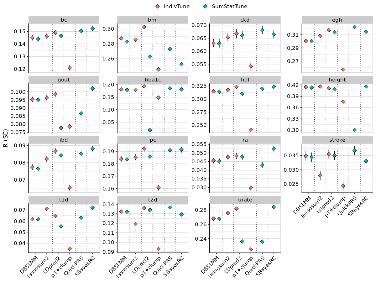
for(pheno_i in selected_traits){
tmp <- res_eval_simp[res_eval_simp$Trait == pheno_i,]
#tmp <- tmp[tmp$Target != 'EUR',]
tmp$Discovery_clean <- as.character(tmp$Discovery)
tmp$Discovery_clean <- paste0(tmp$Discovery_clean, ' GWAS')
tmp$Target <- paste0(tmp$Target, ' Target')
png(paste0('~/oliverpainfel/Analyses/crosspop/plots/', pheno_i,'.png'), res=300, width = 3400, height = 2000, units = 'px')
plot_tmp<-ggplot(tmp, aes(x=label, y=R , fill = Model)) +
geom_errorbar(aes(ymin = R - SE, ymax = R + SE),
width = 0,
position = position_dodge(width = 1)) +
geom_point(stat="identity", position=position_dodge(1), size=3, shape=23) +
geom_vline(xintercept = seq(1.5, length(unique(tmp$label))), linetype="dotted") +
labs(y = "R (SE)", x=NULL, fill = NULL, title = info_all$`Trait Description`[info_all$`Trait Label` == pheno_i]) +
facet_grid(Target ~ Discovery_clean, scales='free', space = 'free_x') +
theme_half_open() +
background_grid(major = 'y', minor = 'y') +
panel_border() +
theme(axis.text.x = element_text(angle = 45, vjust = 1, hjust=1),
legend.position = "top",
legend.key.spacing.x = unit(1, "cm"),
legend.justification = "center")
print(plot_tmp)
dev.off()
}
####
# Average results across phenotypes
####
library(MAd)
# Average R across phenotypes
meta_res_eval <- NULL
for(targ_pop_i in targ_pop){
if(targ_pop_i == 'EAS'){
disc_pop <- 'EAS'
}
if(targ_pop_i == 'AFR'){
disc_pop <- 'AFR'
}
if(targ_pop_i == 'EUR'){
disc_pop <- c('EAS','AFR')
}
for(disc_pop_i in disc_pop){
# Subset res_eval for each scenario
res_eval_i <- do.call(rbind, lapply(seq_along(res_eval), function(i) {
x <- res_eval[[i]]
x$pheno <- names(res_eval)[i]
x <- x[x$Target == targ_pop_i]
x <- x[x$gwas_group == paste0('EUR+', disc_pop_i)]
}))
# Average res_evalults for each test across phenotypes
# Use MAd to account for correlation between them
res_eval_i$Sample<-'A'
for(group_i in unique(res_eval_i$Group)){
res_eval_group_i <- res_eval_i[res_eval_i$Group == group_i,]
missing_pheno <-
colnames(cors[[targ_pop_i]])[!(colnames(cors[[targ_pop_i]]) %in% unique(res_eval_group_i$pheno))]
if (!all(colnames(cors[[targ_pop_i]]) %in% unique(res_eval_group_i$pheno))) {
print(paste0(
'res_evalults missing for ',
targ_pop_i,
' ',
group_i,
' ',
paste0(missing_pheno, collapse = ' ')
))
}
cors_i <- cors[[targ_pop_i]][unique(res_eval_group_i$pheno), unique(res_eval_group_i$pheno)]
meta_res_eval_i <-
agg(
id = Sample,
es = R,
var = SE ^ 2,
cor = cors_i,
method = "BHHR",
mod = NULL,
data = res_eval_group_i
)
tmp <- data.table(Group = group_i,
Method = res_eval_group_i$Method[1],
Model = res_eval_group_i$Model[1],
Source = res_eval_group_i$Source[1],
Discovery = res_eval_group_i$Discovery[1],
gwas_group = res_eval_group_i$gwas_group[1],
Target = targ_pop_i,
R = meta_res_eval_i$es,
SE = sqrt(meta_res_eval_i$var))
meta_res_eval <- rbind(meta_res_eval, tmp)
}
}
}
meta_res_eval$Model<-factor(meta_res_eval$Model, levels=c('IndivTune','SumStatTune','Multi-IndivTune','Multi-SumStatTune'))
meta_res_eval$Discovery<-factor(meta_res_eval$Discovery, levels=c('AFR','EAS','EUR','EUR+AFR','EUR+EAS'))
write.csv(meta_res_eval, '~/oliverpainfel/Analyses/crosspop/r_eval.csv', row.names = F)
# Plot average performance across phenotypes for AFR and EAS targets
tmp <- meta_res_eval
tmp <- tmp[tmp$Target != 'EUR',]
tmp <- merge(tmp, pgs_method_labels, by.x = 'Method', by.y = 'method', all.x = T)
tmp$label[is.na(tmp$label)] <- 'All'
tmp$label[grepl('Multi', tmp$Model) & !(tmp$Method %in% pgs_group_methods) & tmp$label != 'All'] <- paste0(tmp$label[grepl('Multi', tmp$Model) & !(tmp$Method %in% pgs_group_methods) & tmp$label != 'All'], '-multi')
tmp$label <- factor(tmp$label, levels = model_order)
tmp$Discovery_clean <- as.character(tmp$Discovery)
tmp$Discovery_clean[tmp$Discovery == 'EUR'] <- 'EUR GWAS'
tmp$Discovery_clean[tmp$Discovery != 'EUR' & tmp$Source == 'Single'] <- 'Target-matched GWAS'
tmp$Discovery_clean[tmp$Discovery != 'EUR' & tmp$Source == 'Multi'] <- 'Both'
tmp$Discovery_clean <- factor(tmp$Discovery_clean,
levels = c('Target-matched GWAS',
'EUR GWAS',
'Both'))
tmp$Target <- paste0(tmp$Target, ' Target')
tmp$Model[tmp$Model != 'SumStatTune'] <- 'IndivTune'
tmp$Model[tmp$Model == 'SumStatTune'] <- 'SumStatTune'
tmp <- tmp[!duplicated(tmp[, c('label','Target','Discovery_clean','Model'), with=F]),]
png(paste0('~/oliverpainfel/Analyses/crosspop/plots/average_r.png'), res=300, width = 3200, height = 2000, units = 'px')
ggplot(tmp, aes(x=label, y=R , fill = Model)) +
geom_errorbar(aes(ymin = R - SE, ymax = R + SE),
width = 0,
position = position_dodge(width = 1)) +
geom_point(stat="identity", position=position_dodge(1), size=3, shape=23) +
geom_vline(xintercept = seq(1.5, length(unique(tmp$label))), linetype="dotted") +
labs(y = "R (SE)", x='Method') +
facet_grid(Target ~ Discovery_clean, scales='free', space = 'free_x') +
theme_half_open() +
background_grid(major = 'y', minor = 'y') +
panel_border() +
theme(axis.text.x = element_text(angle = 45, vjust = 1, hjust=1),
legend.position = "top",
legend.key.spacing.x = unit(1, "cm"),
legend.justification = "center")
dev.off()
# Plot average performance across phenotypes for EUR using AFR or EAS GWAS
tmp <- meta_res_eval
tmp <- tmp[tmp$Target == 'EUR',]
tmp <- merge(tmp, pgs_method_labels, by.x = 'Method', by.y = 'method', all.x = T)
tmp$label[is.na(tmp$label)] <- 'All'
tmp$label[grepl('Multi', tmp$Model) & !(tmp$Method %in% pgs_group_methods) & tmp$label != 'All'] <- paste0(tmp$label[grepl('Multi', tmp$Model) & !(tmp$Method %in% pgs_group_methods) & tmp$label != 'All'], '-multi')
tmp$label <- factor(tmp$label, levels = model_order)
tmp$Discovery_clean <- as.character(tmp$Discovery)
tmp$Discovery_clean <- paste0(tmp$Discovery_clean, ' GWAS')
tmp$Target <- paste0(tmp$Target, ' Target')
tmp$Model[tmp$Model != 'SumStatTune'] <- 'IndivTune'
tmp$Model[tmp$Model == 'SumStatTune'] <- 'SumStatTune'
tmp <- tmp[!duplicated(tmp[, c('label','Target','Discovery_clean','Model'), with=F]),]
png(paste0('~/oliverpainfel/Analyses/crosspop/plots/average_r_eur.png'), res=300, width = 4000, height = 1500, units = 'px')
ggplot(tmp, aes(x=label, y=R , fill = Model)) +
geom_errorbar(aes(ymin = R - SE, ymax = R + SE),
width = 0,
position = position_dodge(width = 1)) +
geom_point(stat="identity", position=position_dodge(1), size=3, shape=23) +
geom_vline(xintercept = seq(1.5, length(unique(tmp$label))), linetype="dotted") +
labs(y = "R (SE)", x='Method') +
facet_grid(Target ~ Discovery_clean, scales='free', space = 'free_x') +
theme_half_open() +
background_grid(major = 'y', minor = 'y') +
panel_border() +
theme(axis.text.x = element_text(angle = 45, vjust = 1, hjust=1),
legend.position = "top",
legend.key.spacing.x = unit(1, "cm"),
legend.justification = "center")
dev.off()
# Plot performance of -multi models trained using LEOPARD vs using indiv-level data
tmp <- meta_res_eval
tmp <- tmp[tmp$Target != 'EUR',]
tmp <- merge(tmp, pgs_method_labels, by.x = 'Method', by.y = 'method')
tmp$label[grepl('Multi', tmp$Model) & !(tmp$Method %in% pgs_group_methods)] <- paste0(tmp$label[grepl('Multi', tmp$Model) & !(tmp$Method %in% pgs_group_methods)], '-multi')
tmp$label <- factor(tmp$label, levels = unique(tmp$label[order(!(grepl('Multi', tmp$label)), tmp$label)]))
tmp<-tmp[grepl('multi', tmp$label),]
tmp <- tmp[tmp$Model != 'Multi-IndivTune',]
tmp$Model<-as.character(tmp$Model)
tmp$Model[tmp$Model != 'SumStatTune']<-'IndivTune'
tmp$Model[tmp$Model == 'SumStatTune']<-'LEOPARD'
tmp$Target <- paste0(tmp$Target, ' Target')
png(paste0('~/oliverpainfel/Analyses/crosspop/plots/average_r_leopard.png'), res=300, width = 1500, height = 2000, units = 'px')
ggplot(tmp, aes(x=label, y=R , fill = Model)) +
geom_errorbar(aes(ymin = R - SE, ymax = R + SE),
width = 0,
position = position_dodge(width = 1)) +
geom_point(stat="identity", position=position_dodge(1), size=3, shape=23) +
geom_vline(xintercept = seq(1.5, length(unique(tmp$label))), linetype="dotted") +
labs(y = "R (SE)", x='Method') +
facet_grid(Target ~., scales='free', space = 'free_x') +
theme_half_open() +
background_grid(major = 'y', minor = 'y') +
panel_border() +
theme(axis.text.x = element_text(angle = 45, vjust = 1, hjust=1),
legend.position = "top",
legend.key.spacing.x = unit(1, "cm"),
legend.justification = "center")
dev.off()
# Make simplified plot
# Just show performance when using IndivTrain (or SumStat), and Remove 'All' model, with both GWAS.
tmp <- meta_res_eval
tmp <- tmp[tmp$Target != 'EUR',]
tmp <- tmp[tmp$Method != 'all',]
tmp <- tmp[tmp$Source == 'Multi',]
tmp <- merge(tmp, pgs_method_labels, by.x = 'Method', by.y = 'method', all.x = T)
tmp$label[grepl('Multi', tmp$Model) & !(tmp$Method %in% pgs_group_methods) & tmp$label != 'All'] <- paste0(tmp$label[grepl('Multi', tmp$Model) & !(tmp$Method %in% pgs_group_methods) & tmp$label != 'All'], '-multi')
tmp$label <- factor(tmp$label, levels = model_order)
tmp$Discovery_clean <- as.character(tmp$Discovery)
tmp$Discovery_clean[tmp$Discovery == 'EUR'] <- 'EUR GWAS'
tmp$Discovery_clean[tmp$Discovery != 'EUR' & tmp$Source == 'Single'] <- 'Target-matched GWAS'
tmp$Discovery_clean[tmp$Discovery != 'EUR' & tmp$Source == 'Multi'] <- 'Both'
tmp$Discovery_clean <- factor(tmp$Discovery_clean,
levels = c('Target-matched GWAS',
'EUR GWAS',
'Both'))
tmp$Target <- paste0(tmp$Target, ' Target')
tmp$Model[tmp$Model != 'SumStatTune'] <- 'IndivTune'
tmp$Model[tmp$Model == 'SumStatTune'] <- 'SumStatTune'
tmp <- tmp[!duplicated(tmp[, c('label','Target','Discovery_clean','Model'), with=F]),]
tmp<-tmp[tmp$Model == 'IndivTune',]
png(paste0('~/oliverpainfel/Analyses/crosspop/plots/average_r_simple.png'), res=300, width = 3200, height = 2000, units = 'px')
ggplot(tmp, aes(x=label, y=R)) +
geom_errorbar(aes(ymin = R - SE, ymax = R + SE),
width = 0,
position = position_dodge(width = 1)) +
geom_point(stat="identity", position=position_dodge(1), size=3, shape=23, fill = 'black') +
geom_vline(xintercept = seq(1.5, length(unique(tmp$label))), linetype="dotted") +
labs(y = "R (SE)", x='Method') +
facet_grid(Target ~ ., scales='free', space = 'free_x') +
theme_half_open() +
background_grid(major = 'y', minor = 'y') +
panel_border() +
theme(axis.text.x = element_text(angle = 45, vjust = 1, hjust=1))
dev.off()
tmp<-tmp[tmp$Method %in% c('ldpred2','prscsx','xwing'),]
png(paste0('~/oliverpainfel/Analyses/crosspop/plots/average_r_simple_ldpred2.png'), res=300, width = 500, height = 500, units = 'px')
ggplot(tmp, aes(x=label, y=R)) +
geom_errorbar(aes(ymin = R - SE, ymax = R + SE),
width = 0,
position = position_dodge(width = 1)) +
# geom_point(stat="identity", position=position_dodge(1), fill = '#3399FF') +
geom_point(stat="identity", position=position_dodge(1), size=3, shape=23, fill = '#3399FF') +
geom_vline(xintercept = seq(1.5, length(unique(tmp$label))), linetype="dotted") +
labs(y = "R (SE)", x='Method') +
facet_grid(Target ~ ., scales='free', space = 'free_x') +
theme_half_open() +
background_grid(major = 'y', minor = 'y') +
panel_border() +
theme(axis.text.x = element_text(angle = 45, vjust = 1, hjust=1))
dev.off()
####
# Create heatmap showing difference between all methods and models
####
# Create a function to mirror pred_comp results
mirror_comp<-function(x){
x_sym <- x
x_sym$Model_1 <- x$Model_2
x_sym$Model_2 <- x$Model_1
x_sym$Model_1_R <- x$Model_2_R
x_sym$Model_2_R <- x$Model_1_R
x_sym$R_diff <- -x_sym$R_diff
x_mirrored <- rbind(x, x_sym)
x_diag<-data.frame(
Model_1=unique(x_mirrored$Model_1),
Model_2=unique(x_mirrored$Model_1),
Model_1_R=x_mirrored$Model_1_R,
Model_2_R=x_mirrored$Model_1_R,
R_diff=NA,
R_diff_pval=NA
)
x_comp<-rbind(x_mirrored, x_diag)
return(x_comp)
}
# Read in results
targ_pop=c('EUR','EAS','AFR')
res_comp <- list()
for(pheno_i in selected_traits){
res_comp_i<-NULL
for(targ_pop_i in targ_pop){
if(targ_pop_i == 'EAS'){
disc_pop <- 'EAS'
}
if(targ_pop_i == 'AFR'){
disc_pop <- 'AFR'
}
if(targ_pop_i == 'EUR'){
disc_pop <- c('EAS','AFR')
}
for(disc_pop_i in disc_pop){
comp_i <-
fread(
paste0(
'/users/k1806347/oliverpainfel/Analyses/crosspop/',
'targ_',
targ_pop_i,
'.disc_EUR_',
disc_pop_i,
'/',
pheno_i,
'/res.pred_comp.txt'
)
)
comp_i<-mirror_comp(comp_i)
comp_i$Target<-targ_pop_i
comp_i$gwas_group<-paste0('EUR+', disc_pop_i)
res_comp_i<-rbind(res_comp_i, comp_i)
}
}
res_comp[[pheno_i]]<-res_comp_i
}
res_comp_all <- do.call(rbind, lapply(names(res_comp), function(name) {
x <- res_comp[[name]]
x$pheno <- name # Add a new column with the name of the element
x # Return the updated dataframe
}))
# Annotate tests to get order correct
res_comp_all$Method1<-sub('\\..*','',res_comp_all$Model_1)
res_comp_all$Method1<-gsub('-.*','', res_comp_all$Method1)
res_comp_all$Method2<-sub('\\..*','',res_comp_all$Model_2)
res_comp_all$Method2<-gsub('-.*','', res_comp_all$Method2)
find_model<-function(x){
mod <- x
mod[grepl('top1$', x) & !grepl('pseudo', x)] <- 'IndivTune'
mod[grepl('top1$', x) & grepl('pseudo', x)] <- 'SumStatTune'
mod[grepl('multi$', x) & !grepl('pseudo', x)] <- 'Multi-IndivTune'
mod[grepl('multi$', x) & grepl('pseudo', x)] <- 'Multi-SumStatTune'
mod[grepl('_multi', x)] <- 'SumStatTune'
mod[x == 'prscsx.pseudo.multi'] <- 'SumStatTune'
mod[x == 'xwing.pseudo.multi'] <- 'SumStatTune'
return(mod)
}
res_comp_all$Model1<-find_model(res_comp_all$Model_1)
res_comp_all$Model2<-find_model(res_comp_all$Model_2)
res_comp_all$Source1<-ifelse(res_comp_all$Method1 %in% pgs_group_methods | grepl('_multi$', res_comp_all$Method1) | !grepl('AFR|EAS|EUR', res_comp_all$Model_1), 'Multi', 'Single')
res_comp_all$Source2<-ifelse(res_comp_all$Method2 %in% pgs_group_methods | grepl('_multi$', res_comp_all$Method2) | !grepl('AFR|EAS|EUR', res_comp_all$Model_2), 'Multi', 'Single')
for(i in c('EUR','EAS','AFR')){
res_comp_all$Discovery1[grepl(i, res_comp_all$Model_1)] <- i
res_comp_all$Discovery2[grepl(i, res_comp_all$Model_2)] <- i
}
res_comp_all$Discovery1[res_comp_all$Source1 == 'Multi'] <- res_comp_all$gwas_group[res_comp_all$Source1 == 'Multi']
res_comp_all$Discovery2[res_comp_all$Source2 == 'Multi'] <- res_comp_all$gwas_group[res_comp_all$Source2 == 'Multi']
res_comp_all$Method1<-factor(res_comp_all$Method1, levels=unique(res_comp_all$Method1))
res_comp_all$Method2<-factor(res_comp_all$Method2, levels=unique(res_comp_all$Method2))
res_comp_all$Model1<-factor(res_comp_all$Model1, levels=c('IndivTune','SumStatTune','Multi-IndivTune','Multi-SumStatTune'))
res_comp_all$Model2<-factor(res_comp_all$Model2, levels=c('IndivTune','SumStatTune','Multi-IndivTune','Multi-SumStatTune'))
res_comp_all$Discovery1<-factor(res_comp_all$Discovery1, levels=rev(c('AFR','EAS','EUR','EUR+AFR','EUR+EAS')))
res_comp_all$Discovery2<-factor(res_comp_all$Discovery2, levels=c('AFR','EAS','EUR','EUR+AFR','EUR+EAS'))
# Remove IndivTune and Multi-IndivTune model for groups that contain one score (aka QuickPRS and SBayesRC)
res_comp_all <- res_comp_all[
!(res_comp_all$Method1 %in% c('quickprs','sbayesrc') &
res_comp_all$Model1 %in% c('IndivTune','Multi-IndivTune')),]
res_comp_all <- res_comp_all[
!(res_comp_all$Method2 %in% c('quickprs','sbayesrc') &
res_comp_all$Model2 %in% c('IndivTune','Multi-IndivTune')),]
# Remove pseudo model for methods that don't really have one
res_comp_all <- res_comp_all[
!(res_comp_all$Method1 %in% c('ptclump','ptclump_multi') &
res_comp_all$Model1 %in% c('SumStatTune','Multi-SumStatTune')),]
res_comp_all <- res_comp_all[
!(res_comp_all$Method2 %in% c('ptclump','ptclump_multi') &
res_comp_all$Model2 %in% c('SumStatTune','Multi-SumStatTune')),]
# Remove top1 models for PRS-CSx
res_comp_all <- res_comp_all[
!(grepl('prscsx|xwing|_multi', res_comp_all$Method1) &
grepl('top1', res_comp_all$Model_1)),]
res_comp_all <- res_comp_all[
!(grepl('prscsx|xwing|_multi', res_comp_all$Method2) &
grepl('top1', res_comp_all$Model_2)),]
# Remove any comparisons
res_comp_all <- res_comp_all[!duplicated(res_comp_all[, c("Target", "gwas_group", "Method1", "Model1", "Source1", "Discovery1", "Method2", "Model2", "Source2", "Discovery2",'pheno')]),]
res_comp_all$r_diff_rel <- res_comp_all$R_diff / res_comp_all$Model_2_R
# Calculate relative improvement for ldpred2-multi vs ldpred2 as example
tmp_ldpred2 <- res_comp_all[res_comp_all$Model_1 == 'ldpred2.multi' &
grepl('ldpred2-', res_comp_all$Model_2) &
res_comp_all$Target == 'AFR',]
tmp_ldpred2 <- tmp_ldpred2[order(-tmp_ldpred2$Model_2_R),]
tmp_ldpred2 <- tmp_ldpred2[!duplicated(tmp_ldpred2$pheno),]
round(min(tmp_ldpred2$r_diff_rel)*100, 1)
round(max(tmp_ldpred2$r_diff_rel)*100, 1)
tmp_ldpred2 <- res_comp_all[res_comp_all$Model_1 == 'ldpred2.multi' &
grepl('ldpred2-', res_comp_all$Model_2) &
res_comp_all$Target == 'EAS',]
tmp_ldpred2 <- tmp_ldpred2[order(-tmp_ldpred2$Model_2_R),]
tmp_ldpred2 <- tmp_ldpred2[!duplicated(tmp_ldpred2$pheno),]
round(min(tmp_ldpred2$r_diff_rel)*100, 1)
round(max(tmp_ldpred2$r_diff_rel)*100, 1)
# Calculate relative improvement for sbayesrc-multi vs sbayesrc in EUR target as example
tmp_sbayesrc <- res_comp_all[res_comp_all$Model_1 == 'sbayesrc.pseudo.multi' &
grepl('sbayesrc.pseudo-', res_comp_all$Model_2) &
res_comp_all$Target == 'EUR' &
res_comp_all$Discovery1 == 'EUR+EAS' &
res_comp_all$Discovery2 == 'EUR',]
tmp_sbayesrc <- tmp_sbayesrc[order(-tmp_sbayesrc$Model_2_R),]
round(min(tmp_sbayesrc$r_diff_rel)*100, 1)
round(max(tmp_sbayesrc$r_diff_rel)*100, 1)
tmp_sbayesrc <- res_comp_all[res_comp_all$Model_1 == 'sbayesrc.pseudo.multi' &
grepl('sbayesrc.pseudo-', res_comp_all$Model_2) &
res_comp_all$Target == 'EUR' &
res_comp_all$Discovery1 == 'EUR+AFR' &
res_comp_all$Discovery2 == 'EUR',]
tmp_sbayesrc <- tmp_sbayesrc[order(-tmp_sbayesrc$Model_2_R),]
round(min(tmp_sbayesrc$r_diff_rel)*100, 1)
round(max(tmp_sbayesrc$r_diff_rel)*100, 1)
#####
# Export a csv containing difference results for all traits
#####
# Simplify to contain only IndivTune or SumStatTune result
tmp <- res_comp_all
tmp <- merge(tmp, pgs_method_labels, by.x = 'Method1', by.y = 'method', all.x = T)
tmp$label[is.na(tmp$label)] <- 'All'
names(tmp)[names(tmp) == 'label'] <- 'label1'
tmp <- merge(tmp, pgs_method_labels, by.x = 'Method2', by.y = 'method', all.x = T)
tmp$label[is.na(tmp$label)] <- 'All'
names(tmp)[names(tmp) == 'label'] <- 'label2'
tmp$label1[grepl('Multi', tmp$Model1) & !(tmp$Method1 %in% pgs_group_methods) & tmp$label1 != 'All'] <- paste0(tmp$label1[grepl('Multi', tmp$Model1) & !(tmp$Method1 %in% pgs_group_methods) & tmp$label1 != 'All'], '-multi')
tmp$label2[grepl('Multi', tmp$Model2) & !(tmp$Method2 %in% pgs_group_methods) & tmp$label2 != 'All'] <- paste0(tmp$label2[grepl('Multi', tmp$Model2) & !(tmp$Method2 %in% pgs_group_methods) & tmp$label2 != 'All'], '-multi')
tmp$Model1[tmp$Model1 != 'SumStatTune'] <- 'IndivTune'
tmp$Model1[tmp$Model1 == 'SumStatTune'] <- 'SumStatTune'
tmp$Model2[tmp$Model2 != 'SumStatTune'] <- 'IndivTune'
tmp$Model2[tmp$Model2 == 'SumStatTune'] <- 'SumStatTune'
tmp<-tmp[tmp$Model_1 %in% res_eval_simp$Group,]
tmp<-tmp[tmp$Model_2 %in% res_eval_simp$Group,]
tmp$`Model 1` <- paste0(tmp$label1, ' - ', tmp$Model1, ' - ', tmp$Discovery1)
tmp$`Model 2` <- paste0(tmp$label2, ' - ', tmp$Model2, ' - ', tmp$Discovery2)
tmp <- tmp[, c('Target', 'pheno', 'Model 1', 'Model 2', 'Model_1_R', 'Model_2_R', 'R_diff', 'R_diff_pval'), with=F]
names(tmp) <- c('Target', 'Trait','Model 1', 'Model 2', "R (Model 1)", "R (Model 2)", "R difference (Model 1 R - Model 2 R)", "R difference p-value")
tmp<-tmp[order(tmp$Target, tmp$Trait, tmp$`Model 1`, tmp$`Model 2`),]
tmp$`R difference (Model 1 R - Model 2 R)` <- round(tmp$`R difference (Model 1 R - Model 2 R)`, 3)
tmp$`R (Model 1)` <- round(tmp$`R (Model 1)`, 3)
tmp$`R (Model 2)` <- round(tmp$`R (Model 2)`, 3)
write.csv(tmp, '~/oliverpainfel/Analyses/crosspop/r_diff.csv', row.names=F)
###########
library(MAd)
# Average R across phenotypes
meta_res_comp <- NULL
for(targ_pop_i in targ_pop){
if(targ_pop_i == 'EAS'){
disc_pop <- 'EAS'
}
if(targ_pop_i == 'AFR'){
disc_pop <- 'AFR'
}
if(targ_pop_i == 'EUR'){
disc_pop <- c('EAS','AFR')
}
for(disc_pop_i in disc_pop){
# Subset res_comp for each scenario
res_comp_i <- res_comp_all[res_comp_all$Target == targ_pop_i & res_comp_all$gwas_group == paste0('EUR+', disc_pop_i)]
# Calculate diff SE based on p-value
res_comp_i$R_diff_pval[res_comp_i$R_diff == 0] <- 1-0.001
res_comp_i$R_diff_pval[res_comp_i$R_diff_pval == 1]<-1-0.001
res_comp_i$R_diff_z<-qnorm(res_comp_i$R_diff_pval/2)
res_comp_i$R_diff_SE<-abs(res_comp_i$R_diff/res_comp_i$R_diff_z)
# Average results for each test across phenotypes
# Use MAd to account for correlation between them
res_comp_i$Sample<-'A'
res_comp_i$Group <- paste0(res_comp_i$Model_1, '_vs_', res_comp_i$Model_2)
for(group_i in unique(res_comp_i$Group)){
res_comp_group_i <- res_comp_i[res_comp_i$Group == group_i,]
cors_i <- cors[[targ_pop_i]][unique(res_comp_group_i$pheno), unique(res_comp_group_i$pheno)]
if(res_comp_group_i$Model_1[1] != res_comp_group_i$Model_2[1]){
meta_res_comp_i <-
agg(
id = Sample,
es = R_diff,
var = R_diff_SE ^ 2,
cor = cors_i,
method = "BHHR",
mod = NULL,
data = res_comp_group_i
)
tmp <- res_comp_group_i[1,]
tmp$pheno <- NULL
tmp$Model_1_R <-
meta_res_eval$R[meta_res_eval$Group == tmp$Model_1 &
meta_res_eval$Target == targ_pop_i &
meta_res_eval$gwas_group == paste0('EUR+', disc_pop_i)]
tmp$Model_2_R <-
meta_res_eval$R[meta_res_eval$Group == tmp$Model_2 &
meta_res_eval$Target == targ_pop_i &
meta_res_eval$gwas_group == paste0('EUR+', disc_pop_i)]
tmp$R_diff <- meta_res_comp_i$es
tmp$R_diff_SE <- sqrt(meta_res_comp_i$var)
tmp$R_diff_z <- tmp$R_diff / tmp$R_diff_SE
tmp$R_diff_p <- 2*pnorm(-abs(tmp$R_diff_z))
} else {
tmp <- res_comp_group_i[1,]
tmp$pheno <- NULL
tmp$R_diff <- NA
tmp$R_diff_SE <- NA
tmp$R_diff_z <- NA
tmp$R_diff_p <- NA
}
meta_res_comp <- rbind(meta_res_comp, tmp)
}
}
}
meta_res_comp$R_diff_perc <- meta_res_comp$R_diff / meta_res_comp$Model_2_R
# Extract average improvement for ldpred2-multi vs ldpred2 as example
tmp_ldpred2 <- meta_res_comp[meta_res_comp$Model_1 == 'ldpred2.multi' &
grepl('ldpred2-', meta_res_comp$Model_2) &
meta_res_comp$Target == 'AFR',]
tmp_ldpred2 <- tmp_ldpred2[order(-tmp_ldpred2$Model_2_R),]
round(min(tmp_ldpred2$R_diff_perc)*100, 1)
tmp_ldpred2 <- meta_res_comp[meta_res_comp$Model_1 == 'ldpred2.multi' &
grepl('ldpred2-', meta_res_comp$Model_2) &
meta_res_comp$Target == 'EAS',]
tmp_ldpred2 <- tmp_ldpred2[order(-tmp_ldpred2$Model_2_R),]
round(min(tmp_ldpred2$R_diff_perc)*100, 1)
# Extract average improvement for sbayesrc-multi vs sbayesrc in EUR as example
tmp_sbayesrc <- meta_res_comp[meta_res_comp$Model_1 == 'sbayesrc.pseudo.multi' &
grepl('sbayesrc.pseudo', meta_res_comp$Model_2) &
meta_res_comp$Target == 'EUR' &
meta_res_comp$Discovery1 == 'EUR+AFR' &
meta_res_comp$Discovery2 == 'EUR',]
round(tmp_sbayesrc$R_diff_perc*100, 1)
tmp_sbayesrc <- meta_res_comp[meta_res_comp$Model_1 == 'sbayesrc.pseudo.multi' &
grepl('sbayesrc.pseudo', meta_res_comp$Model_2) &
meta_res_comp$Target == 'EUR' &
meta_res_comp$Discovery1 == 'EUR+EAS' &
meta_res_comp$Discovery2 == 'EUR',]
round(tmp_sbayesrc$R_diff_perc*100, 1)
# Extract average improvement for sbayesrc in EUR compared to all model
tmp_sbayesrc <- meta_res_comp[meta_res_comp$Model_2 == 'sbayesrc.pseudo-EUR.top1' &
meta_res_comp$Model_1 == 'all-EUR.top1' &
meta_res_comp$Target == 'AFR',]
round(tmp_sbayesrc$R_diff_perc*100, 1)
tmp_sbayesrc$R_diff_p
tmp_sbayesrc <- meta_res_comp[meta_res_comp$Model_2 == 'sbayesrc.pseudo-EUR.top1' &
meta_res_comp$Model_1 == 'all-EUR.top1' &
meta_res_comp$Target == 'EAS',]
round(tmp_sbayesrc$R_diff_perc*100, 1)
tmp_sbayesrc$R_diff_p
# Compare QuickPRS-Multi vs QuickPRS to evaluate LEOPARD performance
tmp_quickprs <- meta_res_comp[meta_res_comp$Model_1 == 'quickprs_multi.pseudo.multi' &
meta_res_comp$Model_2 == 'quickprs.pseudo.multi' &
meta_res_comp$Target == 'AFR',]
round(min(tmp_quickprs$R_diff_perc)*100, 1)
tmp_quickprs <- meta_res_comp[meta_res_comp$Model_1 == 'quickprs_multi.pseudo.multi' &
meta_res_comp$Model_2 == 'quickprs.pseudo.multi' &
meta_res_comp$Target == 'EAS',]
round(min(tmp_quickprs$R_diff_perc)*100, 1)
# Compare all.multi method to next best method
tmp_all <- meta_res_comp[meta_res_comp$Model_1 == 'all.multi' &
meta_res_comp$Target == 'AFR' &
meta_res_comp$Source2 == 'Multi',]
tmp_all <- tmp_all[order(tmp_all$R_diff),]
tmp_all <- tmp_all[1,]
round(tmp_all$R_diff_perc*100, 1)
tmp_all$R_diff_p
tmp_all <- meta_res_comp[meta_res_comp$Model_1 == 'all.multi' &
meta_res_comp$Target == 'EAS' &
meta_res_comp$Source2 == 'Multi',]
tmp_all <- tmp_all[order(tmp_all$R_diff),]
tmp_all <- tmp_all[1,]
round(tmp_all$R_diff_perc*100, 1)
tmp_all$R_diff_p
# Compare all.multi method to next best method
tmp_all <- meta_res_comp[meta_res_comp$Model_1 == 'all-AFR.top1' &
meta_res_comp$Target == 'AFR' &
meta_res_comp$Discovery1 == 'AFR' &
meta_res_comp$Discovery2 == 'AFR',]
tmp_all <- tmp_all[order(tmp_all$R_diff),]
tmp_all <- tmp_all[1,]
round(tmp_all$R_diff_perc*100, 1)
tmp_all$R_diff_p
tmp_all <- meta_res_comp[meta_res_comp$Model_1 == 'all-EAS.top1' &
meta_res_comp$Target == 'EAS' &
meta_res_comp$Discovery1 == 'EAS' &
meta_res_comp$Discovery2 == 'EAS',]
tmp_all <- tmp_all[order(tmp_all$R_diff),]
tmp_all <- tmp_all[1,]
round(tmp_all$R_diff_perc*100, 1)
tmp_all$R_diff_p
#####
# Export a csv containing difference results for all traits
#####
# Simplify to contain only IndivTune or SumStatTune result
tmp <- meta_res_comp
tmp <- merge(tmp, pgs_method_labels, by.x = 'Method1', by.y = 'method', all.x = T)
tmp$label[is.na(tmp$label)] <- 'All'
names(tmp)[names(tmp) == 'label'] <- 'label1'
tmp <- merge(tmp, pgs_method_labels, by.x = 'Method2', by.y = 'method', all.x = T)
tmp$label[is.na(tmp$label)] <- 'All'
names(tmp)[names(tmp) == 'label'] <- 'label2'
tmp$label1[grepl('Multi', tmp$Model1) & !(tmp$Method1 %in% pgs_group_methods) & tmp$label1 != 'All'] <- paste0(tmp$label1[grepl('Multi', tmp$Model1) & !(tmp$Method1 %in% pgs_group_methods) & tmp$label1 != 'All'], '-multi')
tmp$label2[grepl('Multi', tmp$Model2) & !(tmp$Method2 %in% pgs_group_methods) & tmp$label2 != 'All'] <- paste0(tmp$label2[grepl('Multi', tmp$Model2) & !(tmp$Method2 %in% pgs_group_methods) & tmp$label2 != 'All'], '-multi')
tmp$Model1[tmp$Model1 != 'SumStatTune'] <- 'IndivTune'
tmp$Model1[tmp$Model1 == 'SumStatTune'] <- 'SumStatTune'
tmp$Model2[tmp$Model2 != 'SumStatTune'] <- 'IndivTune'
tmp$Model2[tmp$Model2 == 'SumStatTune'] <- 'SumStatTune'
tmp<-tmp[tmp$Model_1 %in% res_eval_simp$Group,]
tmp<-tmp[tmp$Model_2 %in% res_eval_simp$Group,]
tmp$`Model 1` <- paste0(tmp$label1, ' - ', tmp$Model1, ' - ', tmp$Discovery1)
tmp$`Model 2` <- paste0(tmp$label2, ' - ', tmp$Model2, ' - ', tmp$Discovery2)
tmp$`Percentage change (R difference / Model 2 R)` <- paste0(round(tmp$R_diff_perc * 100, 1), '%')
tmp <- tmp[, c('Target', 'Model 1', 'Model 2', 'Model_1_R', 'Model_2_R', 'R_diff',"Percentage change (R difference / Model 2 R)", 'R_diff_p'), with=F]
names(tmp) <- c('Target','Model 1', 'Model 2', "R (Model 1)", "R (Model 2)", "R difference (Model 1 R - Model 2 R)", "Percentage change (R difference / Model 2 R)", "R difference p-value")
tmp<-tmp[order(tmp$Target, tmp$`Model 1`, tmp$`Model 2`),]
tmp$`R difference (Model 1 R - Model 2 R)` <- round(tmp$`R difference (Model 1 R - Model 2 R)`, 3)
tmp$`R (Model 1)` <- round(tmp$`R (Model 1)`, 3)
tmp$`R (Model 2)` <- round(tmp$`R (Model 2)`, 3)
write.csv(tmp, '~/oliverpainfel/Analyses/crosspop/r_diff_average.csv', row.names=F)
############
# Group differences
meta_res_comp$R_diff_catagory <- cut(
meta_res_comp$R_diff,
breaks = c(-Inf, -0.08, -0.025, -0.002, 0.002, 0.025, 0.08, Inf),
labels = c('< -0.08', '-0.08 - -0.025', '-0.025 - -0.002', '-0.002 - 0.002', '0.002 - 0.025', '0.025 - 0.08', '> 0.08'),
right = FALSE
)
meta_res_comp$R_diff_catagory <- factor(meta_res_comp$R_diff_catagory, levels = rev(levels(meta_res_comp$R_diff_catagory)))
# Assign significance stars
meta_res_comp$indep_star<-' '
meta_res_comp$indep_star[meta_res_comp$R_diff_p < 0.05]<-'*'
meta_res_comp$indep_star[meta_res_comp$R_diff_p < 1e-3]<-'**'
# meta_res_comp$indep_star[meta_res_comp$R_diff_p < 1e-6]<-'***'
meta_res_comp<-meta_res_comp[order(meta_res_comp$Discovery1, meta_res_comp$Discovery2, meta_res_comp$Method1),]
for(targ_pop_i in targ_pop){
if(targ_pop_i == 'EAS'){
disc_pop <- 'EAS'
}
if(targ_pop_i == 'AFR'){
disc_pop <- 'AFR'
}
if(targ_pop_i == 'EUR'){
disc_pop <- c('EAS','AFR')
}
for(disc_pop_i in disc_pop){
tmp <- meta_res_comp[meta_res_comp$Target == targ_pop_i, ]
tmp <- merge(tmp, pgs_method_labels, by.x = 'Method1', by.y = 'method', all.x = T)
tmp$label[is.na(tmp$label)] <- 'All'
names(tmp)[names(tmp) == 'label'] <- 'label1'
tmp <- merge(tmp, pgs_method_labels, by.x = 'Method2', by.y = 'method', all.x = T)
tmp$label[is.na(tmp$label)] <- 'All'
names(tmp)[names(tmp) == 'label'] <- 'label2'
tmp$label1[grepl('Multi', tmp$Model1) & !(tmp$Method1 %in% pgs_group_methods) & tmp$label1 != 'All'] <- paste0(tmp$label1[grepl('Multi', tmp$Model1) & !(tmp$Method1 %in% pgs_group_methods) & tmp$label1 != 'All'], '-multi')
tmp$label2[grepl('Multi', tmp$Model2) & !(tmp$Method2 %in% pgs_group_methods) & tmp$label2 != 'All'] <- paste0(tmp$label2[grepl('Multi', tmp$Model2) & !(tmp$Method2 %in% pgs_group_methods) & tmp$label2 != 'All'], '-multi')
tmp$Model1[tmp$Model1 != 'SumStatTune'] <- 'IndivTune'
tmp$Model1[tmp$Model1 == 'SumStatTune'] <- 'SumStatTune'
tmp$Model2[tmp$Model2 != 'SumStatTune'] <- 'IndivTune'
tmp$Model2[tmp$Model2 == 'SumStatTune'] <- 'SumStatTune'
tmp<-tmp[tmp$Model_1 %in% res_eval_simp$Group,]
tmp<-tmp[tmp$Model_2 %in% res_eval_simp$Group,]
tmp$label1 <- factor(tmp$label1, levels = model_order)
tmp$label2 <- factor(tmp$label2, levels = model_order)
tmp<-tmp[order(tmp$label1, tmp$label2),]
tmp$label1 <- paste0(tmp$label1," (", ifelse(tmp$Model1 == 'SumStatTune', 'ST', 'IT'), ")")
tmp$label2 <- paste0(tmp$label2," (", ifelse(tmp$Model2 == 'SumStatTune', 'ST', 'IT'), ")")
tmp$label1 <- factor(tmp$label1, levels = unique(tmp$label1))
tmp$label2 <- factor(tmp$label2, levels = unique(tmp$label2))
tmp <- tmp[tmp$gwas_group == paste0('EUR+', disc_pop_i), ]
plot_tmp <- ggplot(data = tmp, aes(label2, label1, fill = R_diff_catagory)) +
geom_tile(color = "white", show.legend = TRUE) +
labs(y = 'Test', x = 'Comparison', fill = 'R difference', title = paste0('Target: ', targ_pop_i)) +
facet_grid(Discovery1 ~ Discovery2, scales = 'free', space = 'free', switch="both") +
geom_text(
data = tmp,
aes(label2, label1, label = indep_star),
color = "black",
size = 4,
angle = 0,
vjust = 0.8
) +
scale_fill_brewer(
breaks = levels(tmp$R_diff_catagory),
palette = "RdBu",
drop = F,
na.value = 'grey'
) +
theme_half_open() +
background_grid() +
panel_border() +
theme(axis.text.x = element_text(
angle = 45,
vjust = 1,
hjust = 1
))
png(paste0('~/oliverpainfel/Analyses/crosspop/plots/average_r_diff.Discovery_EUR_', disc_pop_i,'.Target_', targ_pop_i, '.png'), res=300, width = 4400, height = 3200, units = 'px')
print(plot_tmp)
dev.off()
}
}
####
# Plot relative improvement of methods
####
# Use ptclump IndivTune using EUR GWAS as the reference, as provides an interpretable scale
meta_res_comp_ptclump_top1<-meta_res_comp[meta_res_comp$Method2 == 'all' & meta_res_comp$Source2 == 'Multi',]
meta_res_comp_ptclump_top1$reference_point<-F
meta_res_comp_ptclump_top1$reference_point[meta_res_comp_ptclump_top1$Method1 == 'all' & meta_res_comp_ptclump_top1$Source1 == 'Multi']<-T
meta_res_comp_ptclump_top1$R_diff[is.na(meta_res_comp_ptclump_top1$R_diff)]<-0
meta_res_comp_ptclump_top1$Discovery1 <- factor(meta_res_comp_ptclump_top1$Discovery1, levels=rev(levels(meta_res_comp_ptclump_top1$Discovery1)))
res_comp_all_ptclump_top1<-res_comp_all[res_comp_all$Method2 == 'all' & res_comp_all$Source2 == 'Multi',]
res_comp_all_ptclump_top1$Discovery1 <- factor(res_comp_all_ptclump_top1$Discovery1, levels=levels(meta_res_comp_ptclump_top1$Discovery1))
# Create data to plot reference points
meta_res_comp_reference <- meta_res_comp_ptclump_top1
meta_res_comp_reference$R_diff[meta_res_comp_ptclump_top1$reference_point == F] <- NA
meta_res_comp_reference$R_diff_SE [meta_res_comp_ptclump_top1$reference_point == F] <- NA
res_comp_all_ptclump_top1$reference_point<-F
meta_tmp <- meta_res_comp_ptclump_top1
meta_tmp <- merge(meta_tmp, pgs_method_labels, by.x = 'Method1', by.y = 'method', all.x = T)
meta_tmp$label[is.na(meta_tmp$label)] <- 'All'
meta_tmp$label[grepl('Multi', meta_tmp$Model1) & !(meta_tmp$Method1 %in% pgs_group_methods) & meta_tmp$label != 'All'] <- paste0(meta_tmp$label[grepl('Multi', meta_tmp$Model1) & !(meta_tmp$Method1 %in% pgs_group_methods) & meta_tmp$label != 'All'], '-multi')
meta_tmp$label <- factor(meta_tmp$label, levels = model_order)
meta_tmp$Discovery_clean <- as.character(meta_tmp$Discovery1)
meta_tmp$Discovery_clean[meta_tmp$Discovery1 == 'EUR'] <- 'EUR GWAS'
meta_tmp$Discovery_clean[meta_tmp$Discovery1 != 'EUR' & meta_tmp$Source1 == 'Single'] <- 'Target-matched GWAS'
meta_tmp$Discovery_clean[meta_tmp$Discovery1 != 'EUR' & meta_tmp$Source1 == 'Multi'] <- 'Both'
meta_tmp$Discovery_clean <- factor(meta_tmp$Discovery_clean,
levels = c('Target-matched GWAS',
'EUR GWAS',
'Both'))
meta_tmp$Target <- paste0(meta_tmp$Target, ' Target')
meta_tmp$Model1 <- factor(meta_tmp$Model1, levels = c('IndivTune','SumStatTune','Multi-IndivTune','Multi-SumStatTune'))
meta_tmp_ref <- meta_res_comp_reference
meta_tmp_ref <- merge(meta_tmp_ref, pgs_method_labels, by.x = 'Method1', by.y = 'method', all.x = T)
meta_tmp_ref$label[is.na(meta_tmp_ref$label)] <- 'All'
meta_tmp_ref$label[grepl('Multi', meta_tmp_ref$Model1) & !(meta_tmp_ref$Method1 %in% pgs_group_methods) & meta_tmp_ref$label != 'All'] <- paste0(meta_tmp_ref$label[grepl('Multi', meta_tmp_ref$Model1) & !(meta_tmp_ref$Method1 %in% pgs_group_methods) & meta_tmp_ref$label != 'All'], '-multi')
meta_tmp_ref$label <- factor(meta_tmp_ref$label, levels = model_order)
meta_tmp_ref$Discovery_clean <- as.character(meta_tmp_ref$Discovery1)
meta_tmp_ref$Discovery_clean[meta_tmp_ref$Discovery1 == 'EUR'] <- 'EUR GWAS'
meta_tmp_ref$Discovery_clean[meta_tmp_ref$Discovery1 != 'EUR' & meta_tmp_ref$Source1 == 'Single'] <- 'Target-matched GWAS'
meta_tmp_ref$Discovery_clean[meta_tmp_ref$Discovery1 != 'EUR' & meta_tmp_ref$Source1 == 'Multi'] <- 'Both'
meta_tmp_ref$Discovery_clean <- factor(meta_tmp_ref$Discovery_clean,
levels = c('Target-matched GWAS',
'EUR GWAS',
'Both'))
meta_tmp_ref$Target <- paste0(meta_tmp_ref$Target, ' Target')
meta_tmp_ref$Model1 <- factor(meta_tmp_ref$Model1, levels = c('IndivTune','SumStatTune','Multi-IndivTune','Multi-SumStatTune'))
tmp <- res_comp_all_ptclump_top1
tmp <- merge(tmp, pgs_method_labels, by.x = 'Method1', by.y = 'method', all.x = T)
tmp$label[is.na(tmp$label)] <- 'All'
tmp$label[grepl('Multi', tmp$Model1) & !(tmp$Method1 %in% pgs_group_methods) & tmp$label != 'All'] <- paste0(tmp$label[grepl('Multi', tmp$Model1) & !(tmp$Method1 %in% pgs_group_methods) & tmp$label != 'All'], '-multi')
tmp$label <- factor(tmp$label, levels = model_order)
tmp$Discovery_clean <- as.character(tmp$Discovery1)
tmp$Discovery_clean[tmp$Discovery1 == 'EUR'] <- 'EUR GWAS'
tmp$Discovery_clean[tmp$Discovery1 != 'EUR' & tmp$Source1 == 'Single'] <- 'Target-matched GWAS'
tmp$Discovery_clean[tmp$Discovery1 != 'EUR' & tmp$Source1 == 'Multi'] <- 'Both'
tmp$Discovery_clean <- factor(tmp$Discovery_clean,
levels = c('Target-matched GWAS',
'EUR GWAS',
'Both'))
tmp$Target <- paste0(tmp$Target, ' Target')
tmp$Model1 <- factor(tmp$Model1, levels = c('IndivTune','SumStatTune','Multi-IndivTune','Multi-SumStatTune'))
ggplot(meta_tmp, aes(x=label, y=R_diff , fill = Model1)) +
geom_point(
data = tmp,
mapping = aes(x=label, y=R_diff, colour=Model1),
position = position_jitterdodge(jitter.width = 0.2, dodge.width = 0.7),
alpha = 0.3
) +
geom_hline(yintercept = 0) +
geom_errorbar(
aes(
ymin = R_diff - R_diff_SE,
ymax = R_diff + R_diff_SE
),
width = 0,
position = position_dodge(width = 0.7)
) +
geom_point(
stat = "identity",
position = position_dodge(0.7),
size = 3,
shape = 23
) +
geom_point(
data = meta_tmp_ref,
aes(x = label, y = R_diff, fill = Model1),
stat = "identity",
position = position_dodge(0.7), # Ensure same dodge as other points
size = 3, # Increase size for emphasis
shape = 22,
stroke = 1.5,
show.legend=F
) +
geom_vline(xintercept = seq(1.5, length(unique(meta_tmp$label))), linetype="dotted") +
labs(y = "R_diff (SE)") +
facet_grid(Target ~ Discovery_clean, scales='free', space = 'free_x') +
theme_half_open() +
background_grid() +
panel_border() +
theme(axis.text.x = element_text(angle = 45, vjust = 1, hjust=1))
# Plot as % change
meta_tmp$R_diff_perc <- meta_tmp$R_diff / meta_tmp$Model_2_R
meta_tmp_ref$R_diff_perc <- meta_tmp_ref$R_diff / meta_tmp_ref$Model_2_R
tmp$R_diff_perc <- tmp$R_diff / tmp$Model_2_R
meta_tmp$R_diff_perc_SE <- meta_tmp$R_diff_SE / meta_tmp$Model_2_R
library(scales)
ggplot(meta_tmp, aes(x=label, y=R_diff_perc , fill = Model1)) +
geom_point(
data = tmp,
mapping = aes(x=label, y=R_diff_perc, colour=Model1),
position = position_jitterdodge(jitter.width = 0.2, dodge.width = 0.7),
alpha = 0.3
) +
geom_hline(yintercept = 0) +
geom_errorbar(
aes(
ymin = R_diff_perc - R_diff_perc_SE,
ymax = R_diff_perc + R_diff_perc_SE
),
width = 0,
position = position_dodge(width = 0.7)
) +
geom_point(
stat = "identity",
position = position_dodge(0.7),
size = 3,
shape = 23
) +
geom_point(
data = meta_tmp_ref,
aes(x = label, y = R_diff_perc, fill = Model1),
stat = "identity",
position = position_dodge(0.7), # Ensure same dodge as other points
size = 3, # Increase size for emphasis
shape = 22,
stroke = 1.5,
show.legend=F
) +
scale_y_continuous(labels = percent_format()) +
geom_vline(xintercept = seq(1.5, length(unique(meta_tmp$label))), linetype="dotted") +
labs(y = "R diff. (SE)") +
facet_grid(Target ~ Discovery_clean, scales='free', space = 'free_x') +
theme_half_open() +
background_grid() +
panel_border() +
theme(axis.text.x = element_text(angle = 45, vjust = 1, hjust=1))
# Simplify results showing results only with or without training data
meta_tmp_simple <- meta_tmp
meta_tmp_simple$Model1[meta_tmp_simple$Model1 != 'SumStatTune'] <- 'IndivTune'
meta_tmp_simple$Model1[meta_tmp_simple$Model1 == 'SumStatTune'] <- 'SumStatTune'
meta_tmp_simple$Model2[meta_tmp_simple$Model2 != 'SumStatTune'] <- 'IndivTune'
meta_tmp_simple$Model2[meta_tmp_simple$Model2 == 'SumStatTune'] <- 'SumStatTune'
meta_tmp_simple<-meta_tmp_simple[meta_tmp_simple$Model_1 %in% res_eval_simp$Group,]
meta_tmp_simple<-meta_tmp_simple[meta_tmp_simple$Model_2 %in% res_eval_simp$Group,]
meta_tmp_ref_simple <- meta_tmp_ref
meta_tmp_ref_simple$Model1[meta_tmp_ref_simple$Model1 != 'SumStatTune'] <- 'IndivTune'
meta_tmp_ref_simple$Model1[meta_tmp_ref_simple$Model1 == 'SumStatTune'] <- 'SumStatTune'
meta_tmp_ref_simple$Model2[meta_tmp_ref_simple$Model2 != 'SumStatTune'] <- 'IndivTune'
meta_tmp_ref_simple$Model2[meta_tmp_ref_simple$Model2 == 'SumStatTune'] <- 'SumStatTune'
meta_tmp_ref_simple<-meta_tmp_ref_simple[meta_tmp_ref_simple$Model_1 %in% res_eval_simp$Group,]
meta_tmp_ref_simple<-meta_tmp_ref_simple[meta_tmp_ref_simple$Model_2 %in% res_eval_simp$Group,]
tmp_simple <- tmp
tmp_simple$Model1[tmp_simple$Model1 != 'SumStatTune'] <- 'IndivTune'
tmp_simple$Model1[tmp_simple$Model1 == 'SumStatTune'] <- 'SumStatTune'
tmp_simple$Model2[tmp_simple$Model2 != 'SumStatTune'] <- 'IndivTune'
tmp_simple$Model2[tmp_simple$Model2 == 'SumStatTune'] <- 'SumStatTune'
tmp_simple<-tmp_simple[tmp_simple$Model_1 %in% res_eval_simp$Group,]
tmp_simple<-tmp_simple[tmp_simple$Model_2 %in% res_eval_simp$Group,]
# Export plot for manuscript
png('~/oliverpainfel/Analyses/crosspop/plots/average_r.perc_improv.png', width = 3200, height = 2000, res= 300, units = 'px')
ggplot(meta_tmp_simple[meta_tmp_simple$Target != 'EUR Target',], aes(x=label, y=R_diff_perc , fill = Model1)) +
# geom_boxplot(
# data = tmp_simple[tmp_simple$Target != 'EUR Target',],
# mapping = aes(x=label, y=R_diff_perc, colour=Model1),
# position = position_dodge(0.7),
# alpha = 0.3
# ) +
geom_point(
data = tmp_simple[tmp_simple$Target != 'EUR Target',],
mapping = aes(x=label, y=R_diff_perc, colour=Model1),
position = position_jitterdodge(jitter.width = 0.2, dodge.width = 0.7),
alpha = 0.3
) +
geom_hline(yintercept = 0) +
geom_errorbar(
aes(
ymin = R_diff_perc - R_diff_perc_SE,
ymax = R_diff_perc + R_diff_perc_SE
),
width = 0,
position = position_dodge(width = 0.7)
) +
geom_point(
stat = "identity",
position = position_dodge(0.7),
size = 3,
shape = 23
) +
geom_point(
data = meta_tmp_ref_simple[meta_tmp_ref_simple$Target != 'EUR Target',],
aes(x = label, y = R_diff_perc, fill = Model1),
stat = "identity",
position = position_dodge(0.7), # Ensure same dodge as other points
size = 4,
shape = 22,
show.legend=F
) +
geom_vline(xintercept = seq(1.5, length(unique(meta_tmp_simple$label))), linetype="dotted") +
scale_y_continuous(labels = percent_format()) +
labs(y = "Relative Improvement (SE)", fill = NULL, colour = NULL, x = NULL) +
facet_grid(Target ~ Discovery_clean, scales='free', space = 'free_x') +
theme_half_open() +
background_grid(major = 'y', minor = 'y') +
panel_border() +
theme(
axis.text.x = element_text(angle = 45, vjust = 1, hjust = 1), # Increase x-axis labels
legend.position = "top",
legend.key.spacing.x = unit(2, "cm"),
legend.justification = "center"
)
dev.off()
# Plot for EUR
meta_tmp_simple$Discovery_clean <- paste0(meta_tmp_simple$Discovery1,' GWAS')
meta_tmp_ref_simple$Discovery_clean <- paste0(meta_tmp_ref_simple$Discovery1,' GWAS')
tmp_simple$Discovery_clean <- paste0(tmp_simple$Discovery1,' GWAS')
meta_tmp_simple<-meta_tmp_simple[!duplicated(meta_tmp_simple[, c('label', 'Discovery_clean', 'Model1'), with=F]),]
meta_tmp_ref_simple<-meta_tmp_ref_simple[!duplicated(meta_tmp_ref_simple[, c('label', 'Discovery_clean', 'Model1'), with=F]),]
tmp_simple<-tmp_simple[!duplicated(tmp_simple[, c('label', 'Discovery_clean', 'Model1','pheno'), with=F]),]
png('~/oliverpainfel/Analyses/crosspop/plots/average_r_eur.perc_improv.png', width = 4000, height = 1500, res= 300, units = 'px')
ggplot(meta_tmp_simple[meta_tmp_simple$Target == 'EUR Target',], aes(x=label, y=R_diff_perc , fill = Model1)) +
geom_point(
data = tmp_simple[tmp_simple$Target == 'EUR Target',],
mapping = aes(x=label, y=R_diff_perc, colour=Model1),
position = position_jitterdodge(jitter.width = 0.2, dodge.width = 0.7),
alpha = 0.3
) +
geom_hline(yintercept = 0) +
geom_errorbar(
aes(
ymin = R_diff_perc - R_diff_perc_SE,
ymax = R_diff_perc + R_diff_perc_SE
),
width = 0,
position = position_dodge(width = 0.7)
) +
geom_point(
stat = "identity",
position = position_dodge(0.7),
size = 3,
shape = 23
) +
geom_point(
data = meta_tmp_ref_simple[meta_tmp_ref_simple$Target == 'EUR Target',],
aes(x = label, y = R_diff_perc, fill = Model1),
stat = "identity",
position = position_dodge(0.7), # Ensure same dodge as other points
size = 4,
shape = 22,
show.legend=F
) +
geom_vline(xintercept = seq(1.5, length(unique(meta_tmp_simple$label))), linetype="dotted") +
scale_y_continuous(labels = percent_format()) +
labs(y = "Relative Improvement (SE)", fill = NULL, colour = NULL, x = NULL) +
facet_grid(Target ~ Discovery_clean, scales='free', space = 'free_x') +
theme_half_open() +
background_grid(major = 'y', minor = 'y') +
panel_border() +
theme(
axis.text.x = element_text(angle = 45, vjust = 1, hjust = 1), # Increase x-axis labels
legend.position = "top",
legend.key.spacing.x = unit(2, "cm"),
legend.justification = "center"
)
dev.off()
########
# Plot relative improvement of LEOPARD over IndivTune of SumStatTune scores
########
# meta res
meta_res_comp_ref <- meta_res_comp[meta_res_comp$Model2 == 'Multi-SumStatTune',]
meta_res_comp_ref <- meta_res_comp_ref[meta_res_comp_ref$Method1 != 'all' & meta_res_comp_ref$Method2 != 'all',]
meta_res_comp_ref <- meta_res_comp_ref[meta_res_comp_ref$Model1 == 'SumStatTune' & meta_res_comp_ref$Source1 == 'Multi',]
meta_res_comp_ref <- meta_res_comp_ref[gsub('_multi','', meta_res_comp_ref$Method1) == gsub('_multi','', meta_res_comp_ref$Method2),]
meta_res_comp_ref$R_diff_perc <- meta_res_comp_ref$R_diff / meta_res_comp_ref$Model_2_R
meta_res_comp_ref$R_diff_perc_SE <- meta_res_comp_ref$R_diff_SE / meta_res_comp_ref$Model_2_R
meta_res_comp_ref$Discovery_clean <- paste0(meta_res_comp_ref$Discovery1,' GWAS')
meta_res_comp_ref$Discovery_clean[meta_res_comp_ref$Target != 'EUR'] <- 'EUR + Target-matched GWAS'
meta_res_comp_ref <- merge(meta_res_comp_ref, pgs_method_labels, by.x = 'Method1', by.y = 'method', all.x = T)
meta_res_comp_ref$label[grepl('Multi', meta_res_comp_ref$Model1) & !(meta_res_comp_ref$Method1 %in% pgs_group_methods)] <- paste0(meta_res_comp_ref$label[grepl('Multi', meta_res_comp_ref$Model1) & !(meta_res_comp_ref$Method1 %in% pgs_group_methods)], '-multi')
meta_res_comp_ref$label <- factor(meta_res_comp_ref$label, levels = model_order)
meta_res_comp_ref$Target_clean <- paste0(meta_res_comp_ref$Target,' Target')
# trait-specific res
res_comp_all_ref <- res_comp_all[res_comp_all$Model2 == 'Multi-SumStatTune',]
res_comp_all_ref <- res_comp_all_ref[res_comp_all_ref$Method1 != 'all' & res_comp_all_ref$Method2 != 'all',]
res_comp_all_ref <- res_comp_all_ref[res_comp_all_ref$Model1 == 'SumStatTune' & res_comp_all_ref$Source1 == 'Multi',]
res_comp_all_ref <- res_comp_all_ref[gsub('_multi','', res_comp_all_ref$Method1) == gsub('_multi','', res_comp_all_ref$Method2),]
res_comp_all_ref$R_diff_perc <- res_comp_all_ref$R_diff / res_comp_all_ref$Model_2_R
res_comp_all_ref$R_diff_perc_SE <- res_comp_all_ref$R_diff_SE / res_comp_all_ref$Model_2_R
res_comp_all_ref$Discovery_clean <- paste0(res_comp_all_ref$Discovery1,' GWAS')
res_comp_all_ref$Discovery_clean[res_comp_all_ref$Target != 'EUR'] <- 'EUR + Target-matched GWAS'
res_comp_all_ref <- merge(res_comp_all_ref, pgs_method_labels, by.x = 'Method1', by.y = 'method', all.x = T)
res_comp_all_ref$label[grepl('Multi', res_comp_all_ref$Model1) & !(res_comp_all_ref$Method1 %in% pgs_group_methods)] <- paste0(res_comp_all_ref$label[grepl('Multi', res_comp_all_ref$Model1) & !(res_comp_all_ref$Method1 %in% pgs_group_methods)], '-multi')
res_comp_all_ref$label <- factor(res_comp_all_ref$label, levels = model_order)
res_comp_all_ref$Target_clean <- paste0(res_comp_all_ref$Target,' Target')
tmp_meta<-meta_res_comp_ref
tmp_all<-res_comp_all_ref
tmp_meta<-tmp_meta[!(tmp_meta$Method1 %in% c('prscsx','xwing')),]
tmp_meta<-tmp_meta[tmp_meta$Target != 'EUR',]
tmp_all<-tmp_all[!(tmp_all$Method1 %in% c('prscsx','xwing')),]
tmp_all<-tmp_all[tmp_all$Target != 'EUR',]
library(ggrepel)
# plot
png('~/oliverpainfel/Analyses/crosspop/plots/leopard_perc_improv.png', width = 1800, height = 1100, res= 300, units = 'px')
ggplot(tmp_meta, aes(x=label, y=R_diff_perc , fill = Model1)) +
geom_hline(yintercept = 0) +
geom_errorbar(
aes(
ymin = R_diff_perc - R_diff_perc_SE,
ymax = R_diff_perc + R_diff_perc_SE
),
width = 0,
position = position_dodge(width = 0.7)
) +
geom_point(
stat = "identity",
position = position_dodge(0.7),
size = 3,
shape = 23
) +
geom_vline(xintercept = seq(1.5, length(unique(tmp_meta$label))), linetype="dotted") +
scale_y_continuous(labels = percent_format()) +
labs(y = "Relative Difference (SE)", fill = NULL, colour = NULL, x = NULL) +
facet_grid(. ~ Target_clean) +
theme_half_open() +
background_grid(major = 'y', minor = 'y') +
panel_border() +
theme(
axis.text.x = element_text(angle = 45, vjust = 1, hjust = 1), # Increase x-axis labels
legend.position = 'none'
)
dev.off()
# Now compare quickPRS-multi and prs-csx only with trait
tmp_meta<-meta_res_comp_ref
tmp_all<-res_comp_all_ref
tmp_meta<- tmp_meta[tmp_meta$Target != 'EUR' & tmp_meta$Method1 %in% c('quickprs_multi','prscsx'),]
tmp_all<- tmp_all[tmp_all$Target != 'EUR' & tmp_all$Method1 %in% c('quickprs_multi','prscsx'),]
library(ggrepel)
png('~/oliverpainfel/Analyses/crosspop/plots/leopard_perc_improv_restricted.png', width = 1500, height = 1500, res= 300, units = 'px')
ggplot(tmp_meta, aes(x=label, y=R_diff_perc , fill = Model1)) +
geom_point(
data = tmp_all,
mapping = aes(x=label, y=R_diff_perc, colour=Model1),
position = position_jitterdodge(jitter.width = 0.2, dodge.width = 0.7),
alpha = 0.3
) +
geom_hline(yintercept = 0) +
geom_errorbar(
aes(
ymin = R_diff_perc - R_diff_perc_SE,
ymax = R_diff_perc + R_diff_perc_SE
),
width = 0,
position = position_dodge(width = 0.7)
) +
geom_point(
stat = "identity",
position = position_dodge(0.7),
size = 3,
shape = 23
) +
scale_y_continuous(labels = percent_format()) +
labs(y = "Relative Improvement (SE)", fill = NULL, colour = NULL, x = NULL) +
facet_grid(. ~ Target_clean) +
theme_half_open() +
background_grid(major = 'y', minor = 'y') +
panel_border() +
theme(
axis.text.x = element_text(angle = 45, vjust = 1, hjust = 1), # Increase x-axis labels
legend.position = 'none'
) +
geom_text_repel(
data = tmp_all[
tmp_all$R_diff_perc < -0.25,
],
aes(label = pheno), # label as percent with 1 decimal
position = position_dodge(width = 0.7),
size = 3,
min.segment.length = 0,
segment.color = NA,
show.legend = FALSE
)
dev.off()
# It shows PRS-CSx --meta flag is actually does very well, except when the AFR GWAS is very small (~2700).Show average improvement in AFR + EAS
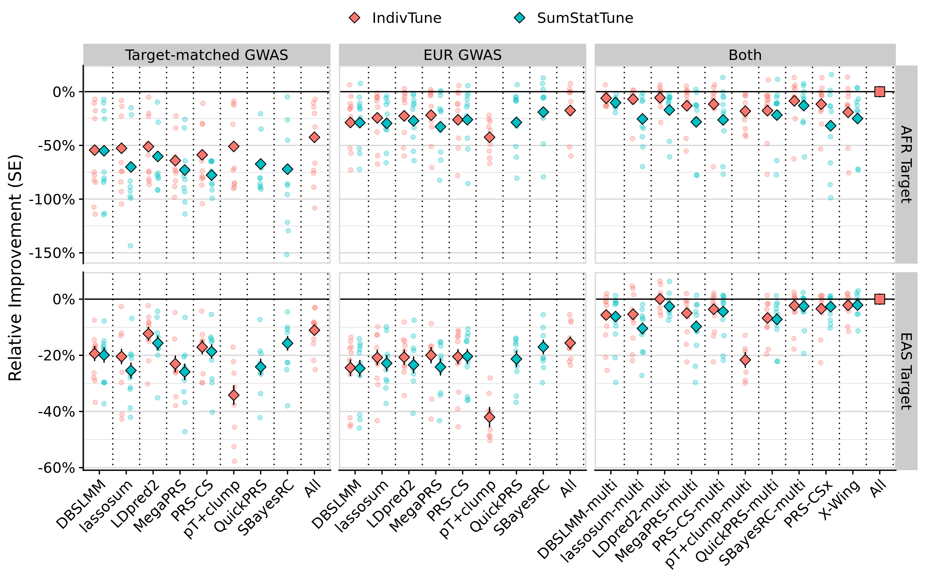
Show average improvement in EUR
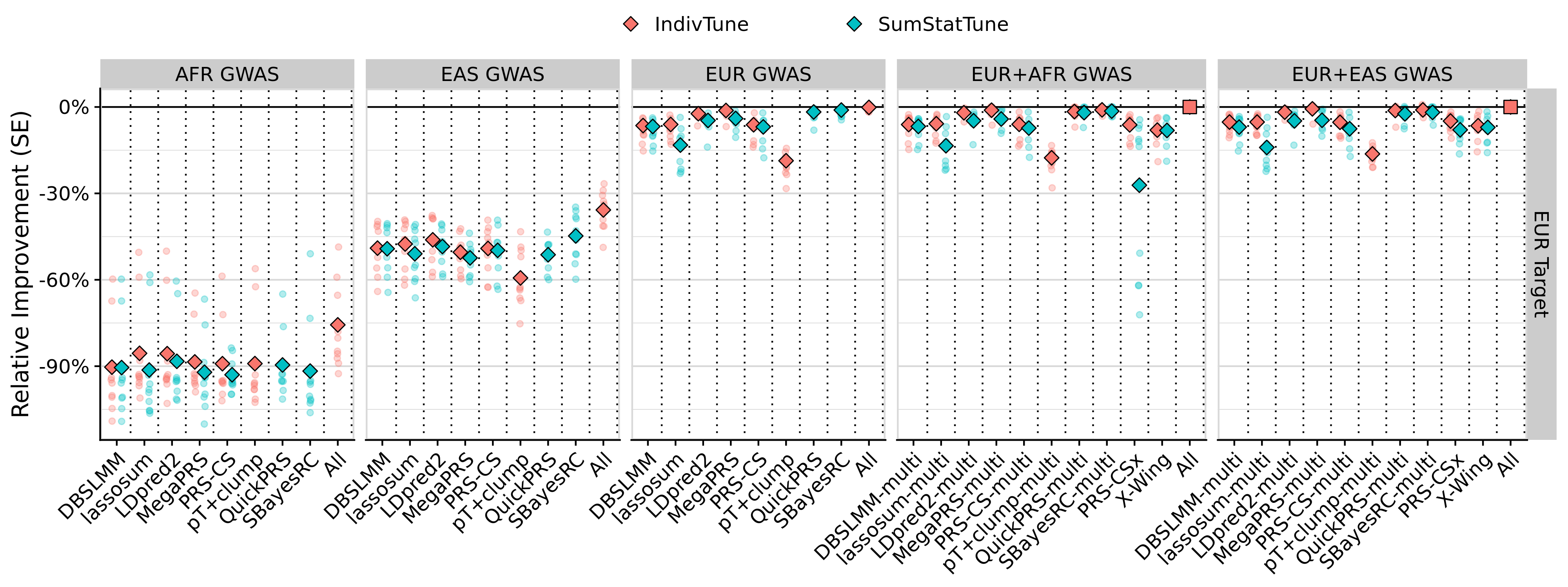
Show LEOPARD comparison
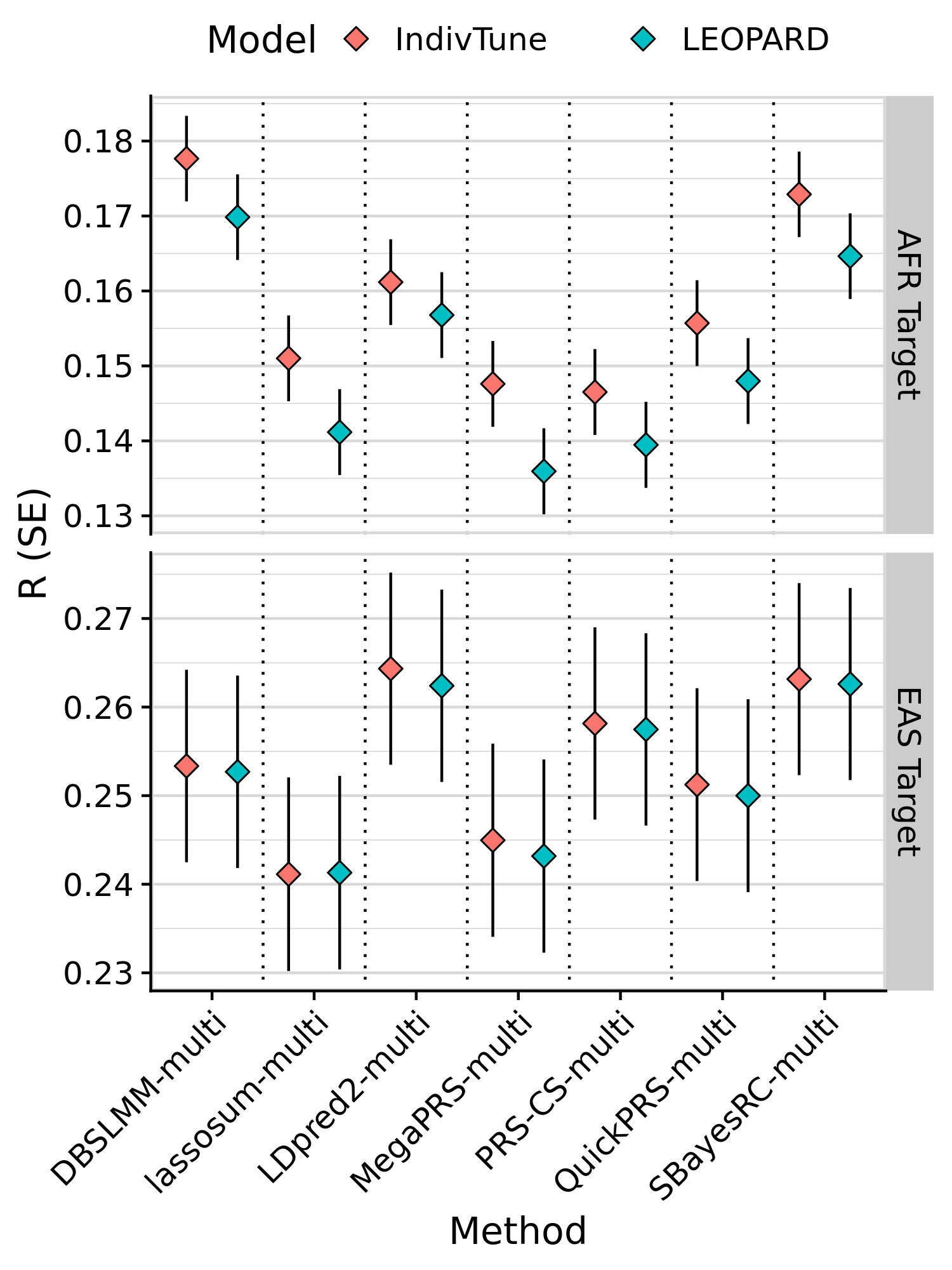
LEOPARD+QuickPRS
Here we will compare the LEOPARD estimated weights for population specific PGS, to the weights estimated using observed data in the UKB target sample.
Show code
setwd('/users/k1806347/oliverpainfel/Software/MyGit/GenoPred/pipeline/')

library(data.table)
library(ggplot2)
library(cowplot)

source('../functions/misc.R')
source_all('../functions')

# Read in list of outcomes
selected_traits<-fread('/users/k1806347/oliverpainfel/Analyses/crosspop/trait_subset.txt', header=F)$V1

# Get some key variables from config
config<-'/users/k1806347/oliverpainfel/Data/ukb/GenoPred/configs/crosspop/config.yaml'
outdir <- read_param(config = config, param = 'outdir', return_obj = F)

# Get a list of score files
scores <- list_score_files(config)

###
# Read in weights estimated by LEOPARD (QuickPRS)
###

leopard_weights<-NULL
scores_quickprs <- scores$name[scores$method == 'quickprs_multi']
for(i in selected_traits){
  scores_i <- scores_quickprs[grepl(paste0('^', i,'_'), scores_quickprs)]
  for(j in scores_i){
      weights_file <- readRDS(paste0(outdir, '/reference/pgs_score_files/leopard/', j, '/ref-', j, '.weights.rds'))
      weights_file <- data.frame(weights_file)

      weights <-
        data.table(
          Target = do.call(c, lapply(names(weights_file), function(x) rep(x, 2))),
          Discovery = names(weights_file),
          Weight = do.call(c, lapply(weights_file, function(x) x)),
          Trait = i,
          Method = 'LEOPARD'
        )

      leopard_weights <- rbind(leopard_weights, weights)
  }
}

#####
# Read in the PGS weights estimated using UKB data
#####
# Read in the final model coefficients for multi-source methods

obs_weights<-NULL
for(method_i in unique(scores$method)[!(unique(scores$method) %in% pgs_group_methods)]){
  scores_method<-scores$name[scores$method == method_i]
  method_i <- gsub('_multi','', method_i)

  for(i in selected_traits){
    for(j in c('EAS','AFR','EUR')){
      if(j == 'EUR'){
        pops <- c('EAS','AFR')
      } else {
        pops <- j
      }

      for(k in pops){
        model <- fread(paste0('~/oliverpainfel/Analyses/crosspop/targ_', j, '.disc_EUR_', k, '/', i, '/final_models/', method_i, '.pseudo.multi.final_model.txt'))
        model<-model[-1,]

        # Set weight to zero if negative, as this is what LEOPARD does
        if(any(model$V2 < 0)){
          model$V2[model$V2 < 0] <- 0
          model$V2[model$V2 > 0] <- 1
        }

        names(model) <- c('x', 'BETA')
        model$Discovery[grepl('UKB', model$x)]<-'EUR'
        model$Discovery[grepl('BBJ', model$x)]<-'EAS'
        model$Discovery[grepl('UGR', model$x)]<-'AFR'
        model$Target <- j
        model$Weight <- model$BETA/sum(model$BETA)
        model$Trait <- i
        model$Method <- method_i
        model<-model[,c('Target','Discovery','Weight','Method','Trait'), with=F]
        obs_weights<-rbind(obs_weights, model)
      }
    }
  }
}

####
## Estimate weights if using the inverse variance weighting (realised this doesn't make sense as PGS are standardised whereas SNP effects in PRS-CSx are not)
####
#
## Read in GWAS descriptives
#gwas_desc<-fread('/users/k1806347/oliverpainfel/Analyses/crosspop/gwas_descriptives.csv')
#gwas_desc <- gwas_desc[, c('Trait Label','Ancestry','GWAS N'), with=F]
#names(gwas_desc)<-c('trait','ancestry','n')
#gwas_desc<-gwas_desc[gwas_desc$trait %in% selected_traits,]
#
#library(dplyr)
#library(tidyr)
#
## Reshape GWAS table to wide format
#wide_gwas <- gwas_desc %>%
#  pivot_wider(names_from = ancestry, values_from = n, values_fill = 0)
#
## Function to create rows for each pair
#make_weights_long <- wide_gwas %>%
#  rowwise() %>%
#  do({
#    trait <- .$trait
#    eur <- .$EUR
#    afr <- .$AFR
#    eas <- .$EAS
#
#    tibble(
#      Trait = trait,
#      Method = "inverse_var",
#      Target = c("AFR", "AFR", "EUR", "EUR", "EUR", "EAS", "EAS"),
#      Discovery = c("EUR", "AFR", "EUR", "AFR", "EAS", "EUR", "EAS"),
#      Weight = c(
#        eur / (eur + afr), afr / (eur + afr),  # AFR target
#        eur / (eur + afr), afr / (eur + afr),  # EUR target (vs AFR)
#        eas / (eur + eas),                     # EUR target (vs EAS)
#        eur / (eur + eas), eas / (eur + eas)   # EAS target (vs EUR)
#      )
#    )
#  }) %>%
#  bind_rows()

###
# Combine and compare
###

#both <- do.call(rbind, list(obs_weights, leopard_weights, make_weights_long))
both <- do.call(rbind, list(obs_weights, leopard_weights))

# Remove ptclump as it doesn't have a sumstattune method
both <- both[both$Method != 'ptclump',]

both<-merge(both, pgs_method_labels, by.x = 'Method', by.y = 'method', all.x=T, sort = F)
both$label[is.na(both$label)] <- both$Method[is.na(both$label)]
both$label <- factor(both$label, levels=unique(both$label))

# Plot non-EUR target first
tmp <- both[both$Target != 'EUR',]
tmp <- tmp[tmp$Discovery != 'EUR',]

# Set LEOPARD to black fill
default_colors <- hue_pal()(10)
names(default_colors) <- levels(tmp$label)
default_colors["LEOPARD"] <- "black"

# Plot the estimated and observed weights
png('~/oliverpainfel/Analyses/crosspop/plots/leopard_weights.png', units = 'px', res = 300, width = 2500, height = 1500)
ggplot(tmp, aes(x = Trait, y = Weight, fill = label)) +
  geom_bar(width= 0.7, position=position_dodge(0.7), stat="identity", colour = 'black', size = 0.1) +
  scale_fill_manual(values = default_colors) +
  facet_grid(Target ~ .) +
  theme_half_open() +
  labs(title = 'Weight of target ancestry-matched PGS', fill = NULL) +
  background_grid(major = 'y', minor = 'y') +
  panel_border() +
  theme(axis.text.x = element_text(angle = 45, hjust = 1)) +
  ylim(c(0,1))
dev.off()

# Plot EUR target
tmp <- both[both$Target == 'EUR',]
tmp <- tmp[tmp$Discovery != 'EUR',]

# Set LEOPARD to black fill
default_colors <- hue_pal()(10)
names(default_colors) <- levels(tmp$label)
default_colors["LEOPARD"] <- "black"

# Plot the estimated and observed weights
png('~/oliverpainfel/Analyses/crosspop/plots/leopard_weights_eur.png', units = 'px', res = 300, width = 2500, height = 1500)
ggplot(tmp, aes(x = Trait, y = Weight, fill = label)) +
  geom_bar(width= 0.7, position=position_dodge(0.7), stat="identity", colour = 'black', size = 0.1) +
  scale_fill_manual(values = default_colors) +
  facet_grid(Discovery ~ .) +
  theme_half_open() +
  labs(title = 'Weight of non-EUR PGS for EUR Target', fill = NULL) +
  background_grid(major = 'y', minor = 'y') +
  panel_border() +
  theme(axis.text.x = element_text(angle = 45, hjust = 1)) +
  ylim(c(0,1))
dev.off()

###
# Check calibration of LEOPARD compared to QuickPRS observed weights
###

tmp <- both[both$Target != 'EUR',]
tmp$Target<-NULL
tmp_wide <- reshape(tmp,
                     idvar = c("Trait", "Discovery"),
                     timevar = "label",
                     direction = "wide")

names(tmp_wide) <- gsub('Weight.', '', names(tmp_wide))
tmp_wide<-tmp_wide[, !(grepl('Method', names(tmp_wide))), with = F]

tmp_wide_eas <- tmp_wide[tmp_wide$Discovery == 'EAS',]
tmp_wide_afr <- tmp_wide[tmp_wide$Discovery == 'AFR',]

# Calculate metrics
rmse_afr <- sqrt(mean((tmp_wide_afr$QuickPRS - tmp_wide_afr$LEOPARD)^2))
me_afr <- mean(tmp_wide_afr$QuickPRS - tmp_wide_afr$LEOPARD)

rmse_eas <- sqrt(mean((tmp_wide_eas$QuickPRS - tmp_wide_eas$LEOPARD)^2))
me_eas <- mean(tmp_wide_eas$QuickPRS - tmp_wide_eas$LEOPARD)

# Create annotation data.frame
metrics_df <- data.frame(
  Discovery = c("AFR", "EAS"),
  x = c(0.5, 0.5),         # Adjust positions as needed
  y = c(-0.05, -0.05),
  label = c(
    paste0("RMSE = ", round(rmse_afr, 2), "\nME = ", round(me_afr, 2)),
    paste0("RMSE = ", round(rmse_eas, 2), "\nME = ", round(me_eas, 2))
  )
)

png('~/oliverpainfel/Analyses/crosspop/plots/leopard_weights_calibration.png', units = 'px', width = 2000, height = 2000, res = 300)
ggplot(tmp_wide[tmp_wide$Discovery != 'EUR',], aes(x = LEOPARD, y = QuickPRS)) +
  geom_abline(slope = 1, intercept = 0, linetype = "dashed", colour = "grey40") +  # Perfect calibration
  geom_smooth(method = "lm", se = TRUE, colour = "blue") +  # Regression line
  geom_point(alpha = 0.7) +
  geom_text(data = metrics_df, aes(x = x, y = y, label = label), inherit.aes = FALSE, hjust = 0, size = 3.5) +
  labs(
    x = "LEOPARD weight",
    y = "Observed weight",
  ) +
  theme_half_open() +
  panel_border() +
  theme(
    axis.text.x = element_text(angle = 90, vjust = 0.5, hjust=1),
  ) +
  facet_grid(. ~ Discovery) +
  coord_fixed()
dev.off()

####
## Check calibration of inverse_var compared to QuickPRS observed weights (again realised this doesn't make sense)
####
#
#tmp <- both[both$Target != 'EUR',]
#tmp$Target<-NULL
#tmp_wide <- reshape(tmp,
#                     idvar = c("Trait", "Discovery"),
#                     timevar = "label",
#                     direction = "wide")
#
#names(tmp_wide) <- gsub('Weight.', '', names(tmp_wide))
#tmp_wide<-tmp_wide[, !(grepl('Method', names(tmp_wide))), with = F]
#
#tmp_wide_eas <- tmp_wide[tmp_wide$Discovery == 'EAS',]
#tmp_wide_afr <- tmp_wide[tmp_wide$Discovery == 'AFR',]
#
## Calculate metrics
#rmse_afr <- sqrt(mean((tmp_wide_afr$QuickPRS - tmp_wide_afr$inverse_var)^2))
#me_afr <- mean(tmp_wide_afr$QuickPRS - tmp_wide_afr$inverse_var)
#
#rmse_eas <- sqrt(mean((tmp_wide_eas$QuickPRS - tmp_wide_eas$inverse_var)^2))
#me_eas <- mean(tmp_wide_eas$QuickPRS - tmp_wide_eas$inverse_var)
#
## Create annotation data.frame
#metrics_df <- data.frame(
#  Discovery = c("AFR", "EAS"),
#  x = c(0.5, 0.5),         # Adjust positions as needed
#  y = c(-0.05, -0.05),
#  label = c(
#    paste0("RMSE = ", round(rmse_afr, 2), "\nME = ", round(me_afr, 2)),
#    paste0("RMSE = ", round(rmse_eas, 2), "\nME = ", round(me_eas, 2))
#  )
#)
#
#png('~/oliverpainfel/Analyses/crosspop/plots/inverse_var_weights_calibration.png', units = 'px', width = 2000, height = 2000, res = 300)
#ggplot(tmp_wide[tmp_wide$Discovery != 'EUR',], aes(x = inverse_var, y = QuickPRS)) +
#  geom_abline(slope = 1, intercept = 0, linetype = "dashed", colour = "grey40") +  # Perfect calibration
#  geom_smooth(method = "lm", se = TRUE, colour = "blue") +  # Regression line
#  geom_point(alpha = 0.7) +
#  geom_text(data = metrics_df, aes(x = x, y = y, label = label), inherit.aes = FALSE, hjust = 1.5, size = 3.5) +
#  labs(
#    x = "inverse_var weight",
#    y = "Observed weight",
#  ) +
#  theme_half_open() +
#  panel_border() +
#  theme(
#    axis.text.x = element_text(angle = 90, vjust = 0.5, hjust=1),
#  ) +
#  facet_grid(. ~ Discovery) +
#  coord_fixed()
#dev.off()

###
# Check calibration of observed weights across all methods
###

tmp <- both[both$Target != 'EUR',]
tmp <- tmp[!(tmp$label %in% c('LEOPARD','inverse_var')),]
tmp$Target<-NULL
tmp_wide <- reshape(tmp,
                     idvar = c("Trait", "Discovery"),
                     timevar = "label",
                     direction = "wide")

names(tmp_wide) <- gsub('Weight.', '', names(tmp_wide))
tmp_wide<-tmp_wide[, !(grepl('Method', names(tmp_wide))), with = F]

tmp_wide <- tmp_wide[tmp_wide$Discovery %in% c('EAS','AFR'),]

metrics <- NULL
for(i in c('EAS','AFR')){
  for(j in unique(tmp$label)){
    for(k in unique(tmp$label)){
      tmp_wide_i <- tmp_wide[tmp_wide$Discovery == i,]
      rmse <- sqrt(mean((tmp_wide_i[[j]] - tmp_wide_i[[k]])^2))
      me <- mean(tmp_wide_i[[j]] - tmp_wide_i[[k]])

      metrics <- rbind(
        metrics,
        data.frame(
          Population = i,
          Method1 = j,
          Method2 = k,
          rmse = rmse,
          me = me
        )
      )
    }
  }
}

png('~/oliverpainfel/Analyses/crosspop/plots/observed_weights_calibration.png', units = 'px', width = 3000, height = 1650, res = 300)
ggplot(metrics, aes(x = Method1, y = Method2, fill = rmse)) +
  geom_tile(color = "white") +  # Tile plot with white borders
  geom_text(aes(label = round(rmse, 2)), color = "black") +  # Add correlation values
  scale_fill_gradient2(mid = "white", high = "red", midpoint = 0) +  # Color scale
  theme_half_open() +
  panel_border() +
  theme(
    axis.text.x = element_text(angle = 45, hjust = 1),
    axis.title = element_blank()
  ) +
  facet_grid(. ~ Population) +
  labs(fill = "RMSE")
dev.off()

# Calculate average RMSE for each method against all other methods
metrics_unique <- metrics[metrics$Method1 != metrics$Method2, ]
metrics_unique$Comparison <- NA
for (i in 1:nrow(metrics_unique)) {
  metrics_unique$Comparison[i] <-
    paste0(sort(c(
      metrics_unique$Method1[i], metrics_unique$Method2[i]
    )), collapse = ' vs. ')
}
metrics_unique <- metrics_unique[!duplicated(paste0(metrics_unique$Population, metrics_unique$Comparison)),]

mean_rmse <- NULL
for(i in unique(tmp$label)){
  for(j in c('AFR','EAS')){
    metrics_unique_tmp <- metrics_unique[metrics_unique$Method1 == i | metrics_unique$Method2 == i,]
    metrics_unique_tmp <- metrics_unique_tmp[metrics_unique_tmp$Population == j,]
    mean_rmse <- rbind(
      mean_rmse,
      data.frame(
        Method = i,
        Population = j,
        avg_rmse = mean(metrics_unique_tmp$rmse)
      )
    )
  }
}

png('~/oliverpainfel/Analyses/crosspop/plots/avg_observed_weight_rmse.png', units = 'px', width = 1500, height = 1500, res = 300)
ggplot(mean_rmse, aes(x = Method, y = avg_rmse, fill = Method)) +
  geom_bar(width= 0.7, position=position_dodge(0.7), stat="identity", size = 0.1) +
  geom_text(aes(label = round(avg_rmse, 3)),  # <-- Add this
          vjust = 1.5,                    # <-- Move the text slightly above the bar
          size = 3) +                      # <-- Adjust text size
  scale_fill_manual(values = default_colors) +
  facet_grid(Population ~ .) +
  theme_half_open() +
  background_grid(major = 'y', minor = 'y') +
  panel_border() +
  labs(y = 'Average RMSE') +
  theme(axis.text.x = element_text(angle = 45, hjust = 1),
        legend.position="none")
dev.off()

####
## Check calibration of estimated (LEOPARD and inverse_var) weights compared to observed QuickPRS weights
####
#
#tmp <- both[both$Target != 'EUR',]
#tmp <- tmp[(tmp$label %in% c('LEOPARD','inverse_var','QuickPRS')),]
#tmp$Target<-NULL
#tmp_wide <- reshape(tmp,
#                     idvar = c("Trait", "Discovery"),
#                     timevar = "label",
#                     direction = "wide")
#
#names(tmp_wide) <- gsub('Weight.', '', names(tmp_wide))
#tmp_wide<-tmp_wide[, !(grepl('Method', names(tmp_wide))), with = F]
#
#tmp_wide <- tmp_wide[tmp_wide$Discovery %in% c('EAS','AFR'),]
#
#metrics <- NULL
#for(i in c('EAS','AFR')){
#  for(j in unique(tmp$label)){
#    for(k in unique(tmp$label)){
#      tmp_wide_i <- tmp_wide[tmp_wide$Discovery == i,]
#      rmse <- sqrt(mean((tmp_wide_i[[j]] - tmp_wide_i[[k]])^2))
#      me <- mean(tmp_wide_i[[j]] - tmp_wide_i[[k]])
#
#      metrics <- rbind(
#        metrics,
#        data.frame(
#          Population = i,
#          Method1 = j,
#          Method2 = k,
#          rmse = rmse,
#          me = me
#        )
#      )
#    }
#  }
#}
#
## Plot the rmse for LEOPARD and inverse_var predicting observed QuickPRS weight
#metrics <- metrics[metrics$Method1 == 'QuickPRS',]
#metrics <- metrics[metrics$Method2 != 'QuickPRS',]
#
#png('~/oliverpainfel/Analyses/crosspop/plots/inverse_var_comp_rmse.png', units = 'px', width = 800, height = 1500, res = 300)
#ggplot(metrics, aes(x = Method2, y = rmse, fill = Method2)) +
#  geom_bar(width= 0.7, position=position_dodge(0.7), stat="identity", size = 0.1) +
#  geom_text(aes(label = round(rmse, 3)),  # <-- Add this
#          vjust = 1.5,                    # <-- Move the text slightly above the bar
#          size = 3) +                      # <-- Adjust text size
#  facet_grid(Population ~ .) +
#  theme_half_open() +
#  background_grid(major = 'y', minor = 'y') +
#  panel_border() +
#  labs(y = 'RMSE relative to QuickPRS', x = 'Method') +
#  theme(axis.text.x = element_text(angle = 45, hjust = 1),
#        legend.position="none")
#dev.off()
Show observed and LEOPARD PGS weights
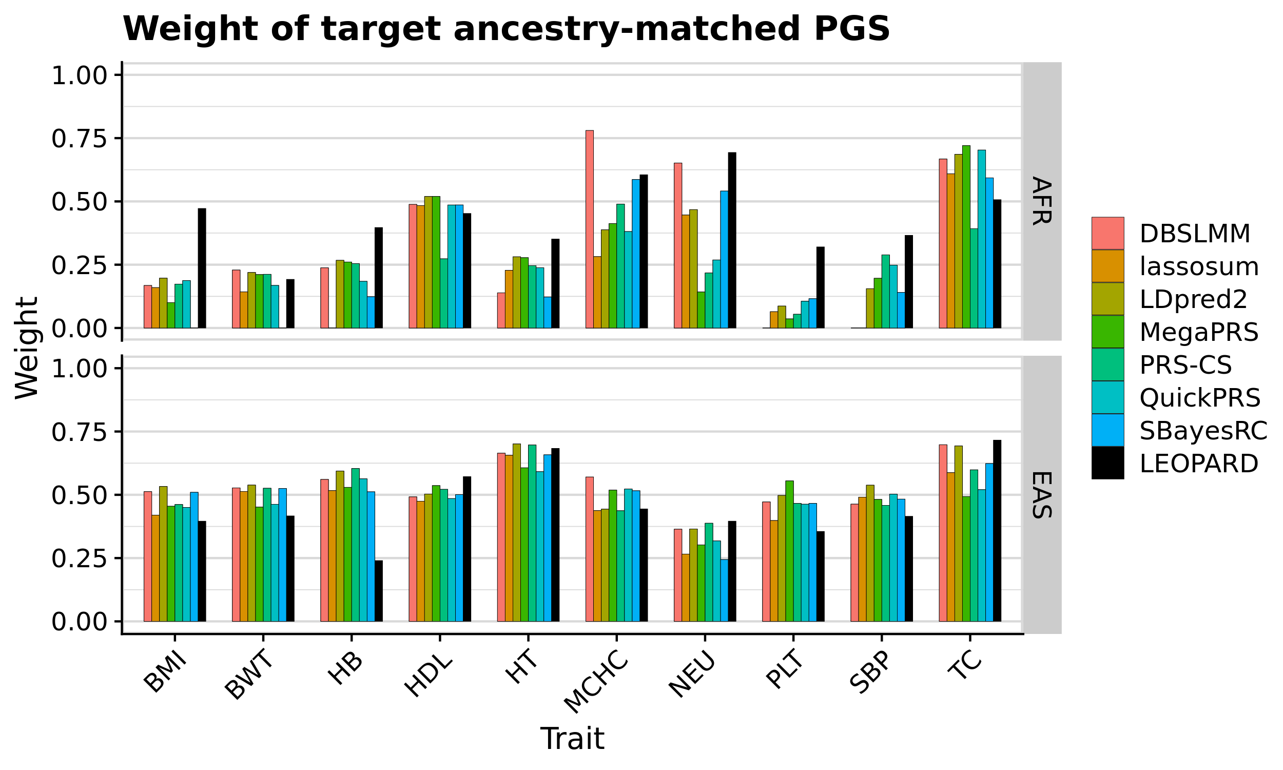
Computational resoures
Here we will read in the benchmark data for PGS methods and create a table for the manuscript.
Show code
library(data.table)
library(ggplot2)
library(cowplot)

setwd('~/oliverpainfel/Software/MyGit/GenoPred/pipeline/')
source('../functions/misc.R')
source_all('../functions')

# Get some key variables from config
config<-'/users/k1806347/oliverpainfel/Data/ukb/GenoPred/configs/crosspop/config.yaml'
pgs_methods <- read_param(config = config, param = 'pgs_methods', return_obj = F)
outdir <- read_param(config = config, param = 'outdir', return_obj = F)

# Read in configuration specific benchmark files
bm_files_i <- list.files(paste0(outdir, '/reference/benchmarks/'), full.names = T)

# Subset benchmarks for pgs_methods
bm_files_i <- bm_files_i[grepl('prep_pgs_|leopard_quickprs_', bm_files_i)]

# Subset to benchmarks for gwas/gwas_groups in config
scores <- list_score_files(config)
bm_files_i <- bm_files_i[grepl(paste0('-', unique(scores$name),'.txt', collapse = '|'), bm_files_i)]

# Read in benchmark files
bm_dat_all <- do.call(rbind, lapply(bm_files_i, function(file) {
  tmp <- fread(file)
  tmp$file <- basename(file)
  return(tmp)
}))

# Create rule column
bm_dat_all$rule <- gsub('-.*','',bm_dat_all$file)

# Create method column
bm_dat_all$method <-
  gsub('_i', '', gsub('prep_pgs_', '', bm_dat_all$rule))

bm_dat_all <- merge(bm_dat_all, pgs_method_labels, by = 'method', all.x=T)

bm_dat_all$label[bm_dat_all$method == 'leopard_quickprs']<-"LEOPARD (QuickPRS)"

#############
# Time
#############

# Calculate average time taken for each method
method_avg <- NULL
for(i in unique(bm_dat_all$label)){
  method_avg <- rbind(
    method_avg,
    data.frame(
      method = bm_dat_all$method[bm_dat_all$label == i][1],
      Method = i,
      Time = mean(bm_dat_all$s[bm_dat_all$label == i])
    )
  )
}

# Times X-Wing time by two since it used 20 cores, but other methods used 10
method_avg$Time[method_avg$method == 'xwing'] <- method_avg$Time[method_avg$method == 'xwing'] * 2

# Divide the multi-source methods (PRS-CSx and X-Wing by 2 so it is time per GWAS)
method_avg$Time[method_avg$method %in% c('prscsx','xwing','leopard_quickprs')] <- method_avg$Time[ method_avg$method %in% c('prscsx','xwing','leopard_quickprs')] / 2

# Approximate times for either tuning or grid only
method_avg$Model <- 'Full'

tmp <- method_avg[method_avg$method == 'prscs' & method_avg$Model == 'Full',]
tmp$Model <- 'auto'
tmp$Time <- tmp$Time * (1/5)
method_avg<-rbind(method_avg, tmp)

tmp <- method_avg[method_avg$method == 'prscsx' & method_avg$Model == 'Full',]
tmp$Model <- 'auto'
tmp$Time <- tmp$Time * (1/5)
method_avg<-rbind(method_avg, tmp)

tmp <- method_avg[method_avg$method == 'xwing' & method_avg$Model == 'Full',]
tmp$Model <- 'grid'
tmp$Time <- tmp$Time * (2/10)
method_avg<-rbind(method_avg, tmp)

# Format the time taken nicely
method_avg$Time_clean[method_avg$Time < 60] <-
  paste0(round(method_avg$Time[method_avg$Time < 60], 1), ' sec')
method_avg$Time_clean[method_avg$Time > 60] <-
  paste0(round(method_avg$Time[method_avg$Time > 60] / 60, 1), ' min')
method_avg$Time_clean[method_avg$Time > 3600] <-
  paste0(round(method_avg$Time[method_avg$Time > 3600] / 60 / 60, 1), ' hr')

# Convert time in seconds to hours
method_avg$Time_hour <- method_avg$Time / 60/60

# Seperate methods by single or multi source
method_avg$Type[!(method_avg$method %in% pgs_group_methods)]<-'Single-source'
method_avg$Type[method_avg$method %in% pgs_group_methods]<-'Multi-source'
method_avg$Type[method_avg$method == 'leopard_quickprs']<-'Tuning'

method_avg$Type<-factor(method_avg$Type, levels = c('Single-source','Multi-source','Tuning'))
method_avg$Method <- factor(method_avg$Method, levels = c("DBSLMM", "lassosum", "LDpred2", "MegaPRS", "PRS-CS", "pT+clump", "QuickPRS", "SBayesRC", "QuickPRS-Multi", "PRS-CSx", "X-Wing","LEOPARD (QuickPRS)"))

ggplot(method_avg, aes(x = Method, y = Time_hour, fill = Model)) +
  geom_bar(stat = "identity", position="dodge") +
  geom_text(aes(label = Time_clean), vjust = 0.5, angle = 90, hjust = -0.2, position = position_dodge(width = 0.9)) +
  labs(x = NULL, y = "Time (hours)") +
  ylim(0, max(method_avg$Time_hour) + (max(method_avg$Time_hour)/5)) +
  facet_grid(~ Type, scales='free', space = 'free_x') +
  theme_half_open() +
  background_grid(major = 'y', minor = 'y') +
  panel_border() +
  theme(axis.text.x = element_text(angle = 45, hjust = 1))

method_avg <- method_avg[method_avg$Model == 'Full',]
method_avg <- method_avg[, c('Method','Time_hour')]
method_avg$Time_hour <- round(method_avg$Time_hour, 2)
names(method_avg)<-c('Method',"Time (hrs)")

#############
# Memory
#############

# Calculate average max_rss for each method
method_avg_mem <- NULL
for(i in unique(bm_dat_all$label)){
  method_avg_mem <- rbind(
    method_avg_mem,
    data.frame(
      method = bm_dat_all$method[bm_dat_all$label == i][1],
      Method = i,
      Memory = mean(bm_dat_all$max_rss[bm_dat_all$label == i])
    )
  )
}

# Divide X-Wing memory by two, since it used 20 cores, but other methods used 10
method_avg_mem$Memory[method_avg_mem$method == 'xwing'] /2

# Format the Memory nicely
method_avg_mem$Memory_clean <-
  paste0(round(method_avg_mem$Memory/1000, 2), ' Gb')

ggplot(method_avg_mem, aes(x = Method, y = Memory, fill = Method)) +
  geom_bar(stat = "identity", position="dodge") +
  geom_text(aes(label = Memory_clean), vjust = -0.5, position = position_dodge(width = 0.9)) +
  labs(x = "PGS Method", y = "Memory (Mb)") +
  theme_half_open() +
  background_grid() +
  theme(axis.text.x = element_text(angle = 45, hjust = 1), legend.position="none")

method_avg_mem$Memory_gb <- method_avg_mem$Memory/1000
method_avg_mem <- method_avg_mem[, c('Method','Memory_gb')]
method_avg_mem$Memory_gb <- round(method_avg_mem$Memory_gb, 2)
names(method_avg_mem)<-c('Method',"Memory (Gb)")

method_avg<-merge(method_avg, method_avg_mem, by = 'Method')

write.csv(method_avg, '~/oliverpainfel/Analyses/crosspop/time_memory.csv', row.names=F)
Show computational resources table
| Method | Time (hrs) | Memory (Gb) |
|---|---|---|
| DBSLMM | 0.15 | 1.15 |
| lassosum | 0.08 | 7.30 |
| LDpred2 | 0.38 | 20.54 |
| LEOPARD (QuickPRS) | 0.23 | 8.03 |
| MegaPRS | 0.72 | 11.92 |
| PRS-CS | 4.40 | 10.57 |
| PRS-CSx | 6.84 | 15.18 |
| pT+clump | 0.02 | 0.83 |
| QuickPRS | 0.06 | 4.41 |
| SBayesRC | 0.38 | 4.40 |
| X-Wing | 34.12 | 48.70 |