Improving interpretability of polygenic scores using only summary statistics

---

This page describes a project investigatin approaches for converting polygenic scores into interpretable information.

Aims:

• Develop method for converting polygenic Z-scores into absolute estimates using summary statistics
• Develop figures to represent absolute risk
• Validate approach for estimating PRS R2/AUC from summary statistics

See here for a preprint describing this work.

---

1 Converting polygenic Z-scores to absolute estimates

To enable correct intepretation of a polygenic score, the variance explained by the polygenic score must be considered. Furthermore, for binary outcomes the population prevelance must be considered, and for continuous outcomes the population mean and SD must be considered. It is possible to convert relative genetic risk into absolute esimates of an outcome when observed data is available, as 23andMe do, by splitting participants into genetic risk quantiles, and then estimating the mean outcome within each quantile. However, observed data is often not available. Here, we use an alternative approach based on summary statistics only alone.

---

1.1 Describe conversion

---

1.1.1 Binary outcomes

To convert a polygenic Z-score into an absolute estimate of risk, we must know the predicitve utility of the polygenic score (AUC), and the prevelance of the outcome in the general population. Then it is possible to estimate the proportion of cases within each polygenic score quantile using bivariate-normal distribution.

Show code

# Thank you for Alex Gillet for her work developing this code.
ccprobs.f <- function(PRS_auc=0.641, prev=0.7463, n_quantile=20){
  
    # Convert AUC into cohen's d
    d <- sqrt(2)*qnorm(PRS_auc)
    
    # Set mean difference between cases and control polygenic scores
    mu_case <- d
    mu_control <- 0
    
    # Estimate mean and variance of polygenic scores across case and control
    varPRS <- prev*(1+(d^2) - (d*prev)^2) + (1-prev)*(1 - (d*prev)^2)
    E_PRS <- d*prev
    
    # Estimate polygenic score quantiles
    by_quant<-1/n_quantile
    p_quant <- seq(by_quant, 1-by_quant, by=by_quant)
    quant_vals_PRS <- rep(0, length(p_quant))
    quant_f_solve <- function(x, prev, d, pq){prev*pnorm(x-d) + (1-prev)*pnorm(x) - pq}
    for(i in 1:length(p_quant)){
        quant_vals_PRS[i] <- unlist(uniroot(quant_f_solve, prev=prev, d=d, pq= p_quant[i], interval=c(-2.5, 2.5), extendInt = "yes", tol=6e-12)$root)
    }
    
    # Create a table for output
    ul_qv_PRS <- matrix(0, ncol=2, nrow=n_quantile)
    ul_qv_PRS[1,1] <- -Inf
    ul_qv_PRS[2:n_quantile,1] <- quant_vals_PRS
    ul_qv_PRS[1:(n_quantile-1),2] <- quant_vals_PRS
    ul_qv_PRS[n_quantile,2] <- Inf
    
    ul_qv_PRS<-cbind(ul_qv_PRS, (ul_qv_PRS[,1:2]-E_PRS)/sqrt(varPRS))
    
    # Estimate case control proportion for each quantile
    prob_quantile_case <- pnorm(ul_qv_PRS[,2], mean = mu_case) - pnorm(ul_qv_PRS[,1], mean = mu_case)
    prob_quantile_control <- pnorm(ul_qv_PRS[,2], mean = mu_control) - pnorm(ul_qv_PRS[,1], mean = mu_control)
    p_case_quantile <- (prob_quantile_case*prev)/by_quant
    p_cont_quantile <- (prob_quantile_control*(1-prev))/by_quant
    
    # Estimate OR comparing each quantile to bottom quantile
    OR <- p_case_quantile/p_cont_quantile
    OR <- OR/OR[1]
    
    # Return output
    out <- cbind(ul_qv_PRS[,3:4],p_cont_quantile, p_case_quantile, OR)
    row.names(out) <- 1:n_quantile
    colnames(out) <- c("q_min", "q_max","p_control", "p_case", "OR")
    
    data.frame(out)
}

---

1.1.2 Continuous outcomes

To convert a polygenic Z-score into an absolute estimate for a trait, we must know the predicitve utility of the polygenic score (R2), and the mean and SD of the outcome in the general population. Then it is possible to estimate the mean and SD of the trait within each polygenic score quantile using a truncated norm model (currently not theory based).

Show code

# Thank you for Alex Gillet for her work developing this code.
mean_sd_quant.f <- function(PRS_R2=0.641, Outcome_mean=1, Outcome_sd=1, n_quantile=20){
  ### PRS quantiles with a continuous phenotype (Y)
  library(tmvtnorm)
  ###
  E_PRS = 0
  SD_PRS = sqrt(1)
  E_phenotype = Outcome_mean
  SD_phenotype = Outcome_sd 

  by_quant<-1/(n_quantile)
  PRS_quantile_bounds <- qnorm(p=seq(0, 1, by=by_quant), mean= E_PRS, sd= SD_PRS)
  lower_PRS_vec <- PRS_quantile_bounds[1:n_quantile]
  upper_PRS_vec <- PRS_quantile_bounds[2:(n_quantile+1)]
  
  mean_vec <- c(E_phenotype, E_PRS)
  sigma_mat <- matrix(sqrt(PRS_R2)*SD_phenotype*SD_PRS, nrow=2, ncol=2)
  sigma_mat[1,1] <- SD_phenotype^2
  sigma_mat[2,2] <- SD_PRS^2
  
  ### mean of phenotype within the truncated PRS distribution
  out_mean_Y <- rep(0, n_quantile)
  ### SD of phenotype within the truncated PRS distribution
  out_SD_Y <- rep(0, n_quantile)
  ### cov of Y and PRS given truncation on PRS
  out_cov_Y_PRS <- rep(0, n_quantile)
  ### SD of PRS given truncation on PRS
  out_SD_PRS <- rep(0, n_quantile)
  ### mean PRS given truncation on PRS
  out_mean_PRS <- rep(0, n_quantile)
  
  for(i in 1:n_quantile){
    distribution_i <- mtmvnorm(mean = mean_vec,
        sigma = sigma_mat,
        lower = c(-Inf, lower_PRS_vec[i]),
        upper = c(Inf, upper_PRS_vec[i]),
        doComputeVariance=TRUE,
        pmvnorm.algorithm=GenzBretz())
        out_mean_Y[i] <- distribution_i$tmean[1]
        out_mean_PRS[i] <- distribution_i$tmean[2]
        out_SD_Y[i] <- sqrt(distribution_i$tvar[1,1])
        out_SD_PRS[i] <- sqrt(distribution_i$tvar[2,2])
        out_cov_Y_PRS[i] <- distribution_i$tvar[1,2]
  }
  
  out<-data.frame(q=1:n_quantile,
             q_min=lower_PRS_vec,
             q_max=upper_PRS_vec,
             x_mean=out_mean_Y,
             x_sd=out_SD_Y)
  
  return(out)

  out_mean_Y
  out_SD_Y
  
  out_mean_PRS
  out_SD_PRS
  out_cov_Y_PRS
}

library(tmvtnorm)

# Create alternative of script that doesn't require simulation
mean_sd_quant.f <- function(PRS_R2=0.641, Outcome_mean=1, Outcome_sd=1, n_quantile=20){
  ### PRS quantiles with a continuous phenotype (Y)
  library(tmvtnorm)
  ###
  E_PRS = 0
  SD_PRS = sqrt(1)
  E_phenotype = Outcome_mean
  SD_phenotype = Outcome_sd 
  n_quantile=20
  
  by_quant<-1/(n_quantile)
  PRS_quantile_bounds <- qnorm(p=seq(0, 1, by=by_quant), mean= E_PRS, sd= SD_PRS)
  lower_PRS_vec <- PRS_quantile_bounds[1:n_quantile]
  upper_PRS_vec <- PRS_quantile_bounds[2:(n_quantile+1)]
  
  mean_vec <- c(E_phenotype, E_PRS)
  sigma_mat <- matrix(sqrt(PRS_R2)*SD_phenotype*SD_PRS, nrow=2, ncol=2)
  sigma_mat[1,1] <- SD_phenotype^2
  sigma_mat[2,2] <- SD_PRS^2
  
  ### mean of phenotype within the truncated PRS distribution
  out_mean_Y <- rep(0, 20)
  ### SD of phenotype within the truncated PRS distribution
  out_SD_Y <- rep(0, 20)
  ### cov of Y and PRS given truncation on PRS
  out_cov_Y_PRS <- rep(0, 20)
  ### SD of PRS given truncation on PRS
  out_SD_PRS <- rep(0, 20)
  ### mean PRS given truncation on PRS
  out_mean_PRS <- rep(0, 20)
  
  for(i in 1:n_quantile){
    distribution_i <- mtmvnorm(mean = mean_vec,
        sigma = sigma_mat,
        lower = c(-Inf, lower_PRS_vec[i]),
        upper = c(Inf, upper_PRS_vec[i]),
        doComputeVariance=TRUE,
        pmvnorm.algorithm=GenzBretz())
        out_mean_Y[i] <- distribution_i$tmean[1]
        out_mean_PRS[i] <- distribution_i$tmean[2]
        out_SD_Y[i] <- sqrt(distribution_i$tvar[1,1])
        out_SD_PRS[i] <- sqrt(distribution_i$tvar[2,2])
        out_cov_Y_PRS[i] <- distribution_i$tvar[1,2]
  }
  
  out<-data.frame(q=1:n_quantile,
             q_min=lower_PRS_vec,
             q_max=upper_PRS_vec,
             x_mean=out_mean_Y,
             x_sd=out_SD_Y)
  
  return(out)

  out_mean_Y
  out_SD_Y
  
  out_mean_PRS
  out_SD_PRS
  out_cov_Y_PRS
}

pdf('~/comp_stand.pdf')
for(i in seq(0.05, 0.95, 0.05)){
sim_res<-PRS_abs_quant2(PRS_R2 = i, Outcome_mean = 0, Outcome_sd = 1, n_quantile = 20)
nosim_res<-mean_sd_quant.f(PRS_R2 = i, Outcome_mean = 0, Outcome_sd = 1, n_quantile = 20)

plot(sim_res$x_mean,nosim_res$x_mean, main=paste0('R2 = ',i))
abline(coef = c(0,1))
}
dev.off()

pdf('~/comp_centre.pdf')
for(i in seq(0.05, 0.95, 0.05)){
sim_res<-PRS_abs_quant2(PRS_R2 = i, Outcome_mean = 0, Outcome_sd = 2, n_quantile = 20)
nosim_res<-mean_sd_quant.f(PRS_R2 = i, Outcome_mean = 0, Outcome_sd = 2, n_quantile = 20)

plot(sim_res$x_mean,nosim_res$x_mean, main=paste0('R2 = ',i))
abline(coef = c(0,1))

plot(sim_res$x_sd,nosim_res$x_sd, main=paste0('R2 = ',i))
abline(coef = c(0,1))

}
dev.off()

pdf('~/comp_scaled.pdf')
for(i in seq(0.05, 0.95, 0.05)){
sim_res<-PRS_abs_quant2(PRS_R2 = i, Outcome_mean = 100, Outcome_sd = 1, n_quantile = 20)
nosim_res<-mean_sd_quant.f(PRS_R2 = i, Outcome_mean = 100, Outcome_sd = 1, n_quantile = 20)

plot(sim_res$x_mean,nosim_res$x_mean, main=paste0('R2 = ',i))
abline(coef = c(0,1))
}
dev.off()

---

1.2 Validate conversion

---

1.2.1 Calculate polygenic scores

pT + clump: Sparse

########
# 1KG ref
########
# Set required variables
. /users/k1806347/brc_scratch/Software/MyGit/GenoPred/config_used/Target_scoring.config
. /users/k1806347/brc_scratch/Software/MyGit/GenoPred/config_used/Pipeline_prep.config

pheno=$(echo Depression Intelligence BMI Height T2D CAD IBD MultiScler RheuArth Breast_Cancer Prostate_Cancer Depression)
gwas=$(echo DEPR07 COLL01 BODY04 HEIG03 DIAB05 COAD01 INFB01 SCLE03 RHEU02 BRCA01 PRCA01)

# Create directory
mkdir -p ${UKBB_output}/PRS_for_interpretation/1KG_ref/pt_clump

# Create file listing GWAS that haven't been processed.
> ${UKBB_output}/PRS_for_interpretation/1KG_ref/pt_clump/todo.txt
for i in $(seq 1 11);do
gwas_i=$(echo ${gwas} | cut -f ${i} -d ' ')
pheno_i=$(echo ${pheno} | cut -f ${i} -d ' ')
if [ ! -f ${UKBB_output}/PRS_for_interpretation/1KG_ref/pt_clump/${gwas_i}/UKBB.subset.w_hm3.${gwas_i}.profiles ]; then
echo ${gwas_i} ${pheno_i} >> ${UKBB_output}/PRS_for_interpretation/1KG_ref/pt_clump/todo.txt
fi
done

# Create shell script to run using sbatch
cat > ${UKBB_output}/PRS_for_interpretation/1KG_ref/pt_clump/sbatch.sh << 'EOF'
#!/bin/sh

#SBATCH -p shared,brc
#SBATCH --mem 5G
#SBATCH -J pt_clump

. /users/k1806347/brc_scratch/Software/MyGit/GenoPred/config_used/Target_scoring.config
. /users/k1806347/brc_scratch/Software/MyGit/GenoPred/config_used/Pipeline_prep.config

gwas=$(awk -v var="$SLURM_ARRAY_TASK_ID" 'NR == var {print $1}' ${UKBB_output}/PRS_for_interpretation/1KG_ref/pt_clump/todo.txt)
pheno=$(awk -v var="$SLURM_ARRAY_TASK_ID" 'NR == var {print $2}' ${UKBB_output}/PRS_for_interpretation/1KG_ref/pt_clump/todo.txt)

echo $gwas
echo $pheno

/users/k1806347/brc_scratch/Software/Rscript.sh /users/k1806347/brc_scratch/Software/MyGit/GenoPred/Scripts/Scaled_polygenic_scorer/Scaled_polygenic_scorer.R \
    --target_plink_chr ${UKBB_output}/Genotype/Harmonised/UKBB.w_hm3.QCd.AllSNP.chr \
    --target_keep ${UKBB_output}/Phenotype/PRS_comp_subset/UKBB.${pheno}.txt \
    --ref_score ${Geno_1KG_dir}/Score_files_for_polygenic/pt_clump/${gwas}/1KGPhase3.w_hm3.${gwas} \
    --ref_scale ${Geno_1KG_dir}/Score_files_for_polygenic/pt_clump/${gwas}/1KGPhase3.w_hm3.${gwas}.EUR.scale \
    --ref_freq_chr ${Geno_1KG_dir}/freq_files/EUR/1KGPhase3.w_hm3.EUR.chr \
    --plink ${plink1_9} \
    --pheno_name ${gwas} \
    --output ${UKBB_output}/PRS_for_interpretation/1KG_ref/pt_clump/${gwas}/UKBB.subset.w_hm3.${gwas}

EOF

sbatch --array 1-$(wc -l ${UKBB_output}/PRS_for_interpretation/1KG_ref/pt_clump/todo.txt | cut -d' ' -f1)%3 ${UKBB_output}/PRS_for_interpretation/1KG_ref/pt_clump/sbatch.sh

DBSLMM

########
# 1KG ref
######## 
# Set required variables
. /users/k1806347/brc_scratch/Software/MyGit/GenoPred/config_used/Target_scoring.config
. /users/k1806347/brc_scratch/Software/MyGit/GenoPred/config_used/Pipeline_prep.config

pheno=$(echo Depression Intelligence BMI Height T2D CAD IBD MultiScler RheuArth Breast_Cancer Prostate_Cancer Depression)
gwas=$(echo DEPR07 COLL01 BODY04 HEIG03 DIAB05 COAD01 INFB01 SCLE03 RHEU02 BRCA01 PRCA01)

# Create directory
mkdir -p ${UKBB_output}/PRS_for_interpretation/1KG_ref/DBSLMM

# Create file listing GWAS that haven't been processed.
> ${UKBB_output}/PRS_for_interpretation/1KG_ref/DBSLMM/todo.txt
for i in $(seq 1 11);do
gwas_i=$(echo ${gwas} | cut -f ${i} -d ' ')
pheno_i=$(echo ${pheno} | cut -f ${i} -d ' ')
if [ ! -f ${UKBB_output}/PRS_for_interpretation/1KG_ref/DBSLMM/${gwas_i}/UKBB.subset.w_hm3.${gwas_i}.DBSLMM_profiles ]; then
echo ${gwas_i} ${pheno_i} >> ${UKBB_output}/PRS_for_interpretation/1KG_ref/DBSLMM/todo.txt
fi
done

# Create shell script to run using sbatch
cat > ${UKBB_output}/PRS_for_interpretation/1KG_ref/DBSLMM/sbatch.sh << 'EOF'
#!/bin/sh

#SBATCH -p shared,brc
#SBATCH --mem 5G
#SBATCH -J DBSLMM

. /users/k1806347/brc_scratch/Software/MyGit/GenoPred/config_used/Target_scoring.config
. /users/k1806347/brc_scratch/Software/MyGit/GenoPred/config_used/Pipeline_prep.config

gwas=$(awk -v var="$SLURM_ARRAY_TASK_ID" 'NR == var {print $1}' ${UKBB_output}/PRS_for_interpretation/1KG_ref/DBSLMM/todo.txt)
pheno=$(awk -v var="$SLURM_ARRAY_TASK_ID" 'NR == var {print $2}' ${UKBB_output}/PRS_for_interpretation/1KG_ref/DBSLMM/todo.txt)

echo $gwas
echo $pheno

/users/k1806347/brc_scratch/Software/Rscript.sh /users/k1806347/brc_scratch/Software/MyGit/GenoPred/Scripts/Scaled_polygenic_scorer_DBSLMM/Scaled_polygenic_scorer_DBSLMM.R \
    --target_plink_chr ${UKBB_output}/Genotype/Harmonised/UKBB.w_hm3.QCd.AllSNP.chr \
    --target_keep ${UKBB_output}/Phenotype/PRS_comp_subset/UKBB.${pheno}.txt \
    --ref_score ${Geno_1KG_dir}/Score_files_for_polygenic/DBSLMM/${gwas}/1KGPhase3.w_hm3.${gwas}.dbslmm.GW.txt \
    --ref_scale ${Geno_1KG_dir}/Score_files_for_polygenic/DBSLMM/${gwas}/1KGPhase3.w_hm3.${gwas}.EUR.scale \
    --ref_freq_chr ${Geno_1KG_dir}/freq_files/EUR/1KGPhase3.w_hm3.EUR.chr \
    --plink ${plink1_9} \
    --pheno_name ${gwas} \
    --output ${UKBB_output}/PRS_for_interpretation/1KG_ref/DBSLMM/${gwas}/UKBB.subset.w_hm3.${gwas}

EOF

sbatch --array 1-$(wc -l ${UKBB_output}/PRS_for_interpretation/1KG_ref/DBSLMM/todo.txt | cut -d' ' -f1)%3 ${UKBB_output}/PRS_for_interpretation/1KG_ref/DBSLMM/sbatch.sh

---

1.2.2 Evaluate polygenic scores

Compare all methods

# Create a file listing the predictors files
source('/users/k1806347/brc_scratch/Software/MyGit/GenoPred/config_used/Target_scoring.config')

pheno<-c('Depression','Intelligence','BMI','Height','T2D','CAD','IBD','MultiScler','RheuArth','Breast_Cancer','Prostate_Cancer')
gwas<-c('DEPR07','COLL01','BODY04','HEIG03','DIAB05','COAD01','INFB01','SCLE03','RHEU02','BRCA01','PRCA01')

for(i in 1:length(pheno)){
  pred_file<-NULL
    
    # pT+clump (sparse)
    pred_file<-rbind(pred_file,data.frame( predictors=paste0(UKBB_output,'/PRS_for_interpretation/1KG_ref/pt_clump/',gwas[i],'/UKBB.subset.w_hm3.',gwas[i],'.profiles'), 
  group='pT+clump'))
    
    # DBSLMM
    pred_file<-rbind(pred_file,data.frame( predictors=paste0(UKBB_output,'/PRS_for_interpretation/1KG_ref/DBSLMM/',gwas[i],'/UKBB.subset.w_hm3.',gwas[i],'.DBSLMM_profiles'),
  group='DBSLMM'))

    # Write out list of predictors with groups
    dir.create(paste0('/scratch/users/k1806347/Analyses/AbsoluteRisk/Measured_AUC_R2/',pheno[i]))
    write.table(pred_file, paste0('/scratch/users/k1806347/Analyses/AbsoluteRisk/Measured_AUC_R2/',pheno[i],'/UKBB.w_hm3.',gwas[i],'.EUR-PRSs.AllMethodComp.predictor_groups'), row.names=F, col.names=T, quote=F)
}

. /users/k1806347/brc_scratch/Software/MyGit/GenoPred/config_used/Target_scoring.config

# Run Model_builder_V2.R
pheno=$(echo Depression Intelligence BMI Height T2D CAD IBD MultiScler RheuArth Breast_Cancer Prostate_Cancer)
gwas=$(echo DEPR07 COLL01 BODY04 HEIG03 DIAB05 COAD01 INFB01 SCLE03 RHEU02 BRCA01 PRCA01)
prev=$(echo 0.15 NA NA NA 0.05 0.03 0.013 0.00164 0.005 0.125 0.125)

# 1KG reference
for i in $(seq 1 11);do
pheno_i=$(echo ${pheno} | cut -f ${i} -d ' ')
gwas_i=$(echo ${gwas} | cut -f ${i} -d ' ')
prev_i=$(echo ${prev} | cut -f ${i} -d ' ')

sbatch --mem 5G -n 1 -p brc,shared /users/k1806347/brc_scratch/Software/Rscript.sh /users/k1806347/brc_scratch/Software/MyGit/GenoPred/Scripts/Model_builder/Model_builder_V2.R \
  --pheno ${UKBB_output}/Phenotype/PRS_comp_subset/UKBB.${pheno_i}.txt \
  --keep /users/k1806347/brc_scratch/Analyses/PRS_comparison/UKBB_outcomes_for_prediction/ukb18177_glanville_post_qc_id_list.UpdateIDs.fam \
  --out /scratch/users/k1806347/Analyses/AbsoluteRisk/Measured_AUC_R2/${pheno_i}/UKBB.w_hm3.${gwas_i}.EUR-PRSs.AllMethodComp \
  --n_core 1 \
  --compare_predictors F \
  --assoc T \
  --outcome_pop_prev ${prev_i} \
  --predictors /scratch/users/k1806347/Analyses/AbsoluteRisk/Measured_AUC_R2/${pheno_i}/UKBB.w_hm3.${gwas_i}.EUR-PRSs.AllMethodComp.predictor_groups
done

---

1.2.3 Binary outcomes

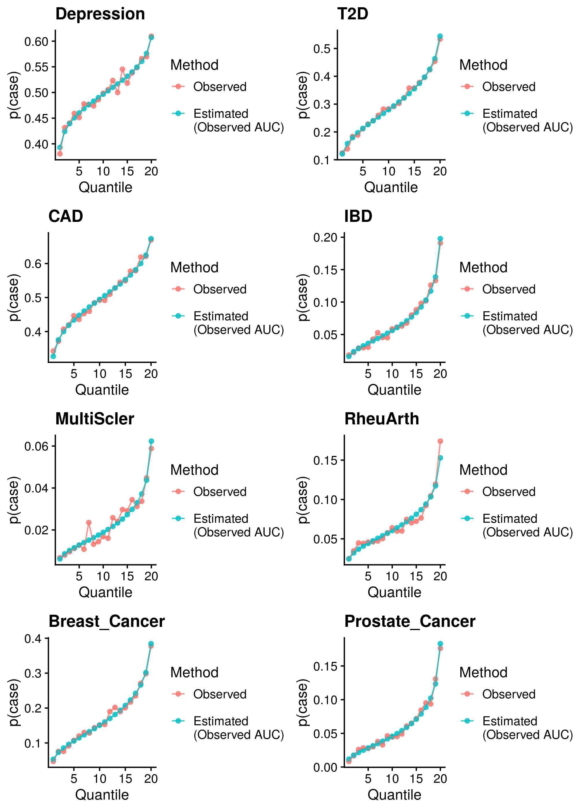
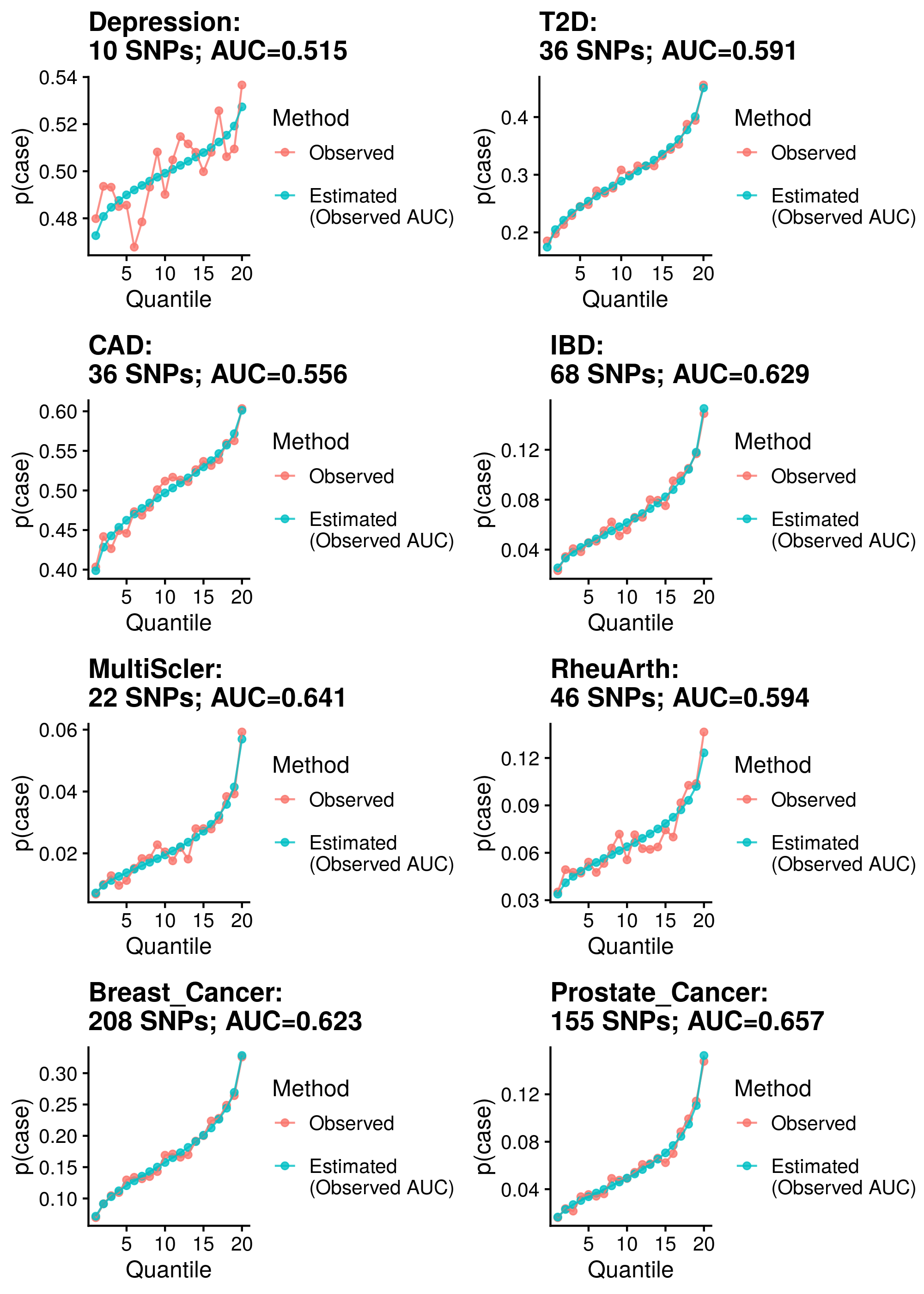
Calculate reference-standardised polygenic scores within UK Biobank for a range of dichotomous phenotypes. Estimate the AUC/R2 of the polygenic scores in UKB. Compare measured and estimated absolute risk per PRS quantile. Use the PRScs fully baysian (pseudovalidation) polygenic scores, as this method provides a single score with good relative performance compared to other approaches.

Reference-standardised polygenic scores have already been calculated in UKB for the PRS methods comparison study, and the AUC has already been estimated. Read in polygenic scores and observed phenotype for UKB, measure proportion of cases per PRS quantile, and then estimate proportion of cases per PRS quantile.

1.2.3.1 DBSLMM

Show code

library(data.table)

source('/users/k1806347/brc_scratch/Software/MyGit/GenoPred/config_used/Target_scoring.config')

pheno=c('Depression','T2D','CAD','IBD','MultiScler','RheuArth','Breast_Cancer','Prostate_Cancer')
gwas=c('DEPR07','DIAB05','COAD01','INFB01','SCLE03','RHEU02','BRCA01','PRCA01')

n_quant<-20

files<-data.frame(pheno,gwas)

# Create function
ccprobs.f <- function(PRS_auc=0.641, prev=0.7463, n_quantile=20){
  
    # Convert AUC into cohen's d
    d <- sqrt(2)*qnorm(PRS_auc)
    
    # Set mean difference between cases and control polygenic scores
    mu_case <- d
    mu_control <- 0
    
    # Estimate mean and variance of polygenic scores across case and control
    varPRS <- prev*(1+(d^2) - (d*prev)^2) + (1-prev)*(1 - (d*prev)^2)
    E_PRS <- d*prev
    
    # Estimate polygenic score quantiles
    by_quant<-1/n_quantile
    p_quant <- seq(by_quant, 1-by_quant, by=by_quant)
    quant_vals_PRS <- rep(0, length(p_quant))
    quant_f_solve <- function(x, prev, d, pq){prev*pnorm(x-d) + (1-prev)*pnorm(x) - pq}
    for(i in 1:length(p_quant)){
        quant_vals_PRS[i] <- unlist(uniroot(quant_f_solve, prev=prev, d=d, pq= p_quant[i], interval=c(-2.5, 2.5), extendInt = "yes", tol=6e-12)$root)
    }
    
    # Create a table for output
    ul_qv_PRS <- matrix(0, ncol=2, nrow=n_quantile)
    ul_qv_PRS[1,1] <- -Inf
    ul_qv_PRS[2:n_quantile,1] <- quant_vals_PRS
    ul_qv_PRS[1:(n_quantile-1),2] <- quant_vals_PRS
    ul_qv_PRS[n_quantile,2] <- Inf
    
    ul_qv_PRS<-cbind(ul_qv_PRS, (ul_qv_PRS[,1:2]-E_PRS)/sqrt(varPRS))
    
    # Estimate case control proportion for each quantile
    prob_quantile_case <- pnorm(ul_qv_PRS[,2], mean = mu_case) - pnorm(ul_qv_PRS[,1], mean = mu_case)
    prob_quantile_control <- pnorm(ul_qv_PRS[,2], mean = mu_control) - pnorm(ul_qv_PRS[,1], mean = mu_control)
    p_case_quantile <- (prob_quantile_case*prev)/by_quant
    p_cont_quantile <- (prob_quantile_control*(1-prev))/by_quant
    
    # Estimate OR comparing each quantile to bottom quantile
    OR <- p_case_quantile/p_cont_quantile
    OR <- OR/OR[1]
    
    # Return output
    out <- cbind(ul_qv_PRS[,3:4],p_cont_quantile, p_case_quantile, OR)
    row.names(out) <- 1:n_quantile
    colnames(out) <- c("q_min", "q_max","p_control", "p_case", "OR")
    
    data.frame(out)
}

# Run analysis for each phenotype
res_all<-NULL
cor_res<-NULL
plots_all<-list()
prs_dist_all<-list()
mean_sd<-NULL

for(i in 1:dim(files)[1]){
  # Read in pheno and prs data, and merge
  pheno_i<-fread(paste0(UKBB_output,'/Phenotype/PRS_comp_subset/UKBB.',files$pheno[i],'.txt'))
  names(pheno_i)[3]<-'pheno'
  prs_i<-fread(paste0(UKBB_output,'/PRS_for_interpretation/1KG_ref/DBSLMM/',files$gwas[i],'/UKBB.subset.w_hm3.',files$gwas[i],'.DBSLMM_profiles'))
  prs_i<-prs_i[,c('FID','IID',paste0(files$gwas[i], '_DBSLMM')), with=F]
  names(prs_i)[3]<-'prs'

  pheno_prs<-merge(pheno_i, prs_i, by=c('FID','IID'))
  
  mean_sd<-rbind(mean_sd,data.frame(Phenotype=files$pheno[i],
                                    Mean_all=mean(pheno_prs$prs),
                                    SD_all=sd(pheno_prs$prs),
                                    Mean_con=mean(pheno_prs$prs[pheno_prs$pheno == 0]),
                                    SD_con=sd(pheno_prs$prs[pheno_prs$pheno == 0]),
                                    Mean_cas=mean(pheno_prs$prs[pheno_prs$pheno == 1]),
                                    SD_cas=sd(pheno_prs$prs[pheno_prs$pheno == 1]),
                                    f_test_pval=var.test(prs ~ pheno, pheno_prs, alternative = "two.sided")$p.value))
  
  # Plot DBSLMM PRS distribution
  library(ggplot2)
  library(cowplot)
  prs_dist_all[[i]]<-ggplot(pheno_prs, aes(x=prs)) +
    geom_histogram() +
    labs(y="Count", x='Polygenic Score', title=files$pheno[i]) +
    theme_cowplot(12)
  
  # Read in AUC for PRS
  assoc<-fread(paste0('/scratch/users/k1806347/Analyses/AbsoluteRisk/Measured_AUC_R2/',files$pheno[i],'/UKBB.w_hm3.',files$gwas[i],'.EUR-PRSs.AllMethodComp.assoc.txt'))
  prs_auc<-assoc[grepl('DBSLMM', assoc$Predictor),]$AUC
  
  # Assign individuals to observed PRS quantiles
  obs_quant<-quantile(pheno_prs$prs, prob = seq(0, 1, length = n_quant+1))
  pheno_prs$obs_quant<-as.numeric(cut( pheno_prs$prs, obs_quant, include.lowest = T))

  # Calculate proportion of each quantile that are cases
  obs_cc<-NULL
  for(k in 1:n_quant){
    obs_cc<-rbind(obs_cc, data.frame(Phenotype=files$pheno[i],
                                     Type='Observed',
                                     Quantile=k,
                                     q_min=obs_quant[k],
                                     q_max=obs_quant[k+1],
                                     p_control=1-mean(pheno_prs$pheno[pheno_prs$obs_quant == k]),
                                     p_case=mean(pheno_prs$pheno[pheno_prs$obs_quant == k])))
  }
  
  # Assign individuals to estimated PRS quantiles
  est_cc<-ccprobs.f(PRS_auc = prs_auc, prev=mean(pheno_prs$pheno), n_quantile = n_quant)
  est_cc$OR<-NULL
  est_cc<-data.frame(Phenotype=files$pheno[i],Type="\nEstimated\n(Observed AUC)",Quantile=1:n_quant, est_cc)
  est_quant<-sort(unique(c(est_cc$q_min, est_cc$q_max)))
  pheno_prs$est_quant<-as.numeric(cut( pheno_prs$prs, est_quant, include.lowest = T))
  
  tmp<-cor.test(obs_cc$p_case, est_cc$p_case)
  tmp2<-abs(est_cc$p_case-obs_cc$p_case)/obs_cc$p_case
  
  # Estimate correlation between observed and expected
  cor_res<-rbind(cor_res,data.frame(Phenotype=files$pheno[i],
                                    Cor=tmp$estimate,
                                    Low95CI=tmp$conf.int[1],
                                    High95CI=tmp$conf.int[2],
                                    Mean_perc_diff=mean(tmp2),
                                    N=length(pheno_prs$pheno),
                                    Ncas=sum(pheno_prs$pheno == 1),
                                    Ncon=sum(pheno_prs$pheno == 0)))

  quant_comp<-rbind(obs_cc, est_cc)
  
  res_all<-rbind(res_all, quant_comp)
  
  library(ggplot2)
  library(cowplot)
  
  plots_all[[i]]<-ggplot(quant_comp, aes(x=Quantile, y=p_case, colour=Type)) +
                    geom_point(alpha=0.8) +
                    geom_line(alpha=0.8) +
                    labs(y="p(case)", title=files$pheno[i], colour='Method') +
                    theme_cowplot(12)
}

png(paste0('/scratch/users/k1806347/Analyses/AbsoluteRisk/Measured_AUC_R2/PRS_dist_binary.png'), units='px', res=300, width=2000, height=2800)
  plot_grid(plotlist=prs_dist_all, ncol = 2)
dev.off()

png(paste0('/scratch/users/k1806347/Analyses/AbsoluteRisk/Measured_AUC_R2/PropCC_Comp.png'), units='px', res=300, width=2000, height=2800)
  plot_grid(plotlist=plots_all, ncol = 2)
dev.off()

write.csv(cor_res, '/scratch/users/k1806347/Analyses/AbsoluteRisk/Measured_AUC_R2/PropCC_Comp.csv', row.names=F, quote=F)

write.csv(mean_sd, '/scratch/users/k1806347/Analyses/AbsoluteRisk/Measured_AUC_R2/PRS_Mean_SD.csv', row.names=F, quote=F)

Show results

Correlation between observed and estimated proportion of cases within polygenic score quantiles

Phenotype	Correlation (95%CI)	Mean Abs. Diff.	N	Ncas	Ncon
Depression	0.985 (0.961-0.994)	1.5%	49999	24999	25000
T2D	0.997 (0.992-0.999)	2.4%	49999	14888	35111
CAD	0.994 (0.985-0.998)	1.5%	49999	25000	24999
IBD	0.994 (0.985-0.998)	6.8%	49999	3461	46538
MultiScler	0.969 (0.922-0.988)	12.6%	49999	1137	48862
RheuArth	0.981 (0.952-0.993)	6.8%	49999	3408	46591
Breast_Cancer	0.995 (0.987-0.998)	4.6%	49999	8512	41487
Prostate_Cancer	0.994 (0.984-0.998)	8.7%	50000	2927	47073

Median Cor. = 0.994053; Mean Cor. = 0.9886512; Min. Cor. = 0.9691668; Max. Cor. = 0.9968126 Mean Abs. Diff = 0.05621957; Min. Mean Abs. Diff. = 0.01504855; Max. Mean Abs. Diff. = 0.1262171

---

1.2.3.2 pT+clump

Show code

library(data.table)

source('/users/k1806347/brc_scratch/Software/MyGit/GenoPred/config_used/Target_scoring.config')

pheno=c('Depression','T2D','CAD','IBD','MultiScler','RheuArth','Breast_Cancer','Prostate_Cancer')
gwas=c('DEPR07','DIAB05','COAD01','INFB01','SCLE03','RHEU02','BRCA01','PRCA01')

n_quant<-20

files<-data.frame(pheno,gwas)

# Create function
ccprobs.f <- function(PRS_auc=0.641, prev=0.7463, n_quantile=20){
  
    # Convert AUC into cohen's d
    d <- sqrt(2)*qnorm(PRS_auc)
    
    # Set mean difference between cases and control polygenic scores
    mu_case <- d
    mu_control <- 0
    
    # Estimate mean and variance of polygenic scores across case and control
    varPRS <- prev*(1+(d^2) - (d*prev)^2) + (1-prev)*(1 - (d*prev)^2)
    E_PRS <- d*prev
    
    # Estimate polygenic score quantiles
    by_quant<-1/n_quantile
    p_quant <- seq(by_quant, 1-by_quant, by=by_quant)
    quant_vals_PRS <- rep(0, length(p_quant))
    quant_f_solve <- function(x, prev, d, pq){prev*pnorm(x-d) + (1-prev)*pnorm(x) - pq}
    for(i in 1:length(p_quant)){
        quant_vals_PRS[i] <- unlist(uniroot(quant_f_solve, prev=prev, d=d, pq= p_quant[i], interval=c(-2.5, 2.5), extendInt = "yes", tol=6e-12)$root)
    }
    
    # Create a table for output
    ul_qv_PRS <- matrix(0, ncol=2, nrow=n_quantile)
    ul_qv_PRS[1,1] <- -Inf
    ul_qv_PRS[2:n_quantile,1] <- quant_vals_PRS
    ul_qv_PRS[1:(n_quantile-1),2] <- quant_vals_PRS
    ul_qv_PRS[n_quantile,2] <- Inf
    
    ul_qv_PRS<-cbind(ul_qv_PRS, (ul_qv_PRS[,1:2]-E_PRS)/sqrt(varPRS))
    
    # Estimate case control proportion for each quantile
    prob_quantile_case <- pnorm(ul_qv_PRS[,2], mean = mu_case) - pnorm(ul_qv_PRS[,1], mean = mu_case)
    prob_quantile_control <- pnorm(ul_qv_PRS[,2], mean = mu_control) - pnorm(ul_qv_PRS[,1], mean = mu_control)
    p_case_quantile <- (prob_quantile_case*prev)/by_quant
    p_cont_quantile <- (prob_quantile_control*(1-prev))/by_quant
    
    # Estimate OR comparing each quantile to bottom quantile
    OR <- p_case_quantile/p_cont_quantile
    OR <- OR/OR[1]
    
    # Return output
    out <- cbind(ul_qv_PRS[,3:4],p_cont_quantile, p_case_quantile, OR)
    row.names(out) <- 1:n_quantile
    colnames(out) <- c("q_min", "q_max","p_control", "p_case", "OR")
    
    data.frame(out)
}

# Run analysis for each phenotype
res_all<-NULL
cor_res<-NULL
plots_all<-list()
prs_dist_all<-list()

for(i in 1:dim(files)[1]){
  # Read in pheno and prs data, and merge
  pheno_i<-fread(paste0(UKBB_output,'/Phenotype/PRS_comp_subset/UKBB.',files$pheno[i],'.txt'))
  names(pheno_i)[3]<-'pheno'
  prs_i<-fread(paste0(UKBB_output,'/PRS_for_interpretation/1KG_ref/pt_clump/',files$gwas[i],'/UKBB.subset.w_hm3.',files$gwas[i],'.profiles'))
  # Extract PRS with the most stringent p-value threshold
  score_nsnp<-fread(paste0('/users/k1806347/brc_scratch/Data/1KG/Phase3/Score_files_for_polygenic/pt_clump/',gwas[i],'/1KGPhase3.w_hm3.',gwas[i],'.NSNP_per_pT'))
  score_nsnp<-score_nsnp[score_nsnp$NSNP >= 5,]
  nsnp<-score_nsnp$NSNP[score_nsnp$pT1 == min(score_nsnp$pT1)]
  pT<-min(score_nsnp$pT1)
  prs_i<-prs_i[,c('FID','IID',paste0(files$gwas[i], '_',pT)), with=F]
  names(prs_i)[3]<-'prs'

  pheno_prs<-merge(pheno_i, prs_i, by=c('FID','IID'))
  
  # Plot DBSLMM PRS distribution
  library(ggplot2)
  library(cowplot)
  prs_dist_all[[i]]<-ggplot(pheno_prs, aes(x=prs)) +
    geom_histogram() +
    labs(y="Count", x='Polygenic Score', title=paste0(files$pheno[i],': ',nsnp,' SNPs')) +
    theme_cowplot(12)
  
  # Read in AUC for PRS
    assoc<-fread(paste0('/scratch/users/k1806347/Analyses/AbsoluteRisk/Measured_AUC_R2/',files$pheno[i],'/UKBB.w_hm3.',files$gwas[i],'.EUR-PRSs.AllMethodComp.assoc.txt'))
    prs_auc<-assoc[grepl(paste0(gwas[i],'_',gsub('-','.',pT)), assoc$Predictor),]$AUC
  
  # Assign individuals to observed PRS quantiles
  obs_quant<-quantile(pheno_prs$prs, prob = seq(0, 1, length = n_quant+1))
  pheno_prs$obs_quant<-as.numeric(cut( pheno_prs$prs, obs_quant, include.lowest = T))

  # Calculate proportion of each quantile that are cases
  obs_cc<-NULL
  for(k in 1:n_quant){
    obs_cc<-rbind(obs_cc, data.frame(Phenotype=files$pheno[i],
                                     Type='Observed',
                                     Quantile=k,
                                     q_min=obs_quant[k],
                                     q_max=obs_quant[k+1],
                                     p_control=1-mean(pheno_prs$pheno[pheno_prs$obs_quant == k]),
                                     p_case=mean(pheno_prs$pheno[pheno_prs$obs_quant == k])))
  }
  
  # Assign individuals to estimated PRS quantiles
  est_cc<-ccprobs.f(PRS_auc = prs_auc, prev=mean(pheno_prs$pheno), n_quantile = n_quant)
  est_cc$OR<-NULL
  est_cc<-data.frame(Phenotype=files$pheno[i],Type="\nEstimated\n(Observed AUC)",Quantile=1:n_quant, est_cc)
  est_quant<-sort(unique(c(est_cc$q_min, est_cc$q_max)))
  pheno_prs$est_quant<-as.numeric(cut( pheno_prs$prs, est_quant, include.lowest = T))
  
  tmp<-cor.test(obs_cc$p_case, est_cc$p_case)
  tmp2<-abs(est_cc$p_case-obs_cc$p_case)/obs_cc$p_case
  
  # Estimate correlation between observed and expected
  cor_res<-rbind(cor_res,data.frame(Phenotype=files$pheno[i],
                                    Cor=tmp$estimate,
                                    Low95CI=tmp$conf.int[1],
                                    High95CI=tmp$conf.int[2],
                                    Mean_perc_diff=mean(tmp2),
                                    N=length(pheno_prs$pheno),
                                    Ncas=sum(pheno_prs$pheno == 1),
                                    Ncon=sum(pheno_prs$pheno == 0)))

  quant_comp<-rbind(obs_cc, est_cc)
  
  res_all<-rbind(res_all, quant_comp)
  
  library(ggplot2)
  library(cowplot)
  
  plots_all[[i]]<-ggplot(quant_comp, aes(x=Quantile, y=p_case, colour=Type)) +
                    geom_point(alpha=0.8) +
                    geom_line(alpha=0.8) +
                    labs(y="p(case)", title=paste0(files$pheno[i],': \n',nsnp,' SNPs; AUC=',round(prs_auc,3)), colour='Method') +
                    theme_cowplot(12)
}

png(paste0('/scratch/users/k1806347/Analyses/AbsoluteRisk/Measured_AUC_R2/pt_clump_PRS_dist_binary.png'), units='px', res=300, width=2000, height=2800)
  plot_grid(plotlist=prs_dist_all, ncol = 2)
dev.off()

png(paste0('/scratch/users/k1806347/Analyses/AbsoluteRisk/Measured_AUC_R2/pt_clump_PropCC_Comp.png'), units='px', res=300, width=2000, height=2800)
  plot_grid(plotlist=plots_all, ncol = 2)
dev.off()

write.csv(cor_res, '/scratch/users/k1806347/Analyses/AbsoluteRisk/Measured_AUC_R2/pt_clump_PropCC_Comp.csv', row.names=F, quote=F)

Show results

Correlation between observed and estimated proportion of cases within polygenic score quantiles

Phenotype	Correlation (95%CI)	Mean Abs. Diff.	N	Ncas	Ncon
Depression	0.779 (0.513-0.908)	1.8%	49999	24999	25000
T2D	0.993 (0.983-0.997)	2.3%	49999	14888	35111
CAD	0.983 (0.956-0.993)	1.6%	49999	25000	24999
IBD	0.99 (0.974-0.996)	6%	49999	3461	46538
MultiScler	0.981 (0.95-0.992)	10.4%	49999	1137	48862
RheuArth	0.951 (0.878-0.981)	9.5%	49999	3408	46591
Breast_Cancer	0.995 (0.987-0.998)	3.3%	49999	8512	41487
Prostate_Cancer	0.992 (0.98-0.997)	6.6%	50000	2927	47073

Median Cor. = 0.9863451; Mean Cor. = 0.9579612; Min. Cor. = 0.7786503; Max. Cor. = 0.9948055

---

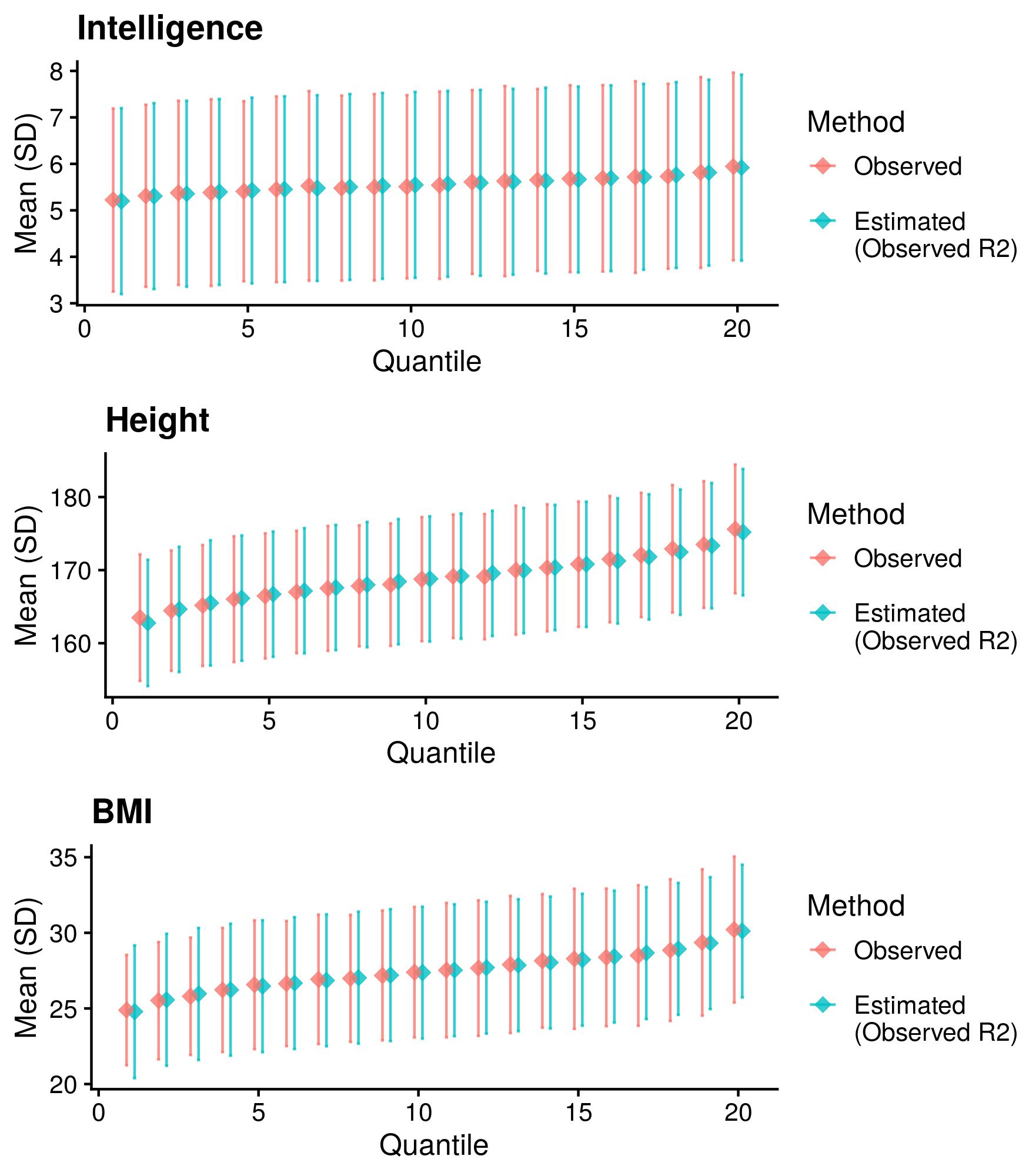
1.2.4 Continuous outcomes

Calculate reference-standardised polygenic scores within UK Biobank for a range of continuous phenotypes. Estimate the R2 of the polygenic scores in UKB. Compare measured and estimated absolute meana and sd per PRS quantile. Use the DBSLMM fully baysian (pseudovalidation) polygenic scores, as this method provides a single score with good relative performance compared to other approaches.

Reference-standardised polygenic scores have already been calculated in UKB for the PRS methods comparison study, and the R2 has already been estimated. Read in polygenic scores and observed phenotype for UKB, measure phenotype mean and sd per PRS quantile, and then estimate measure phenotype mean and sd per PRS quantile.

1.2.4.1 DBSLMM

Show code

library(data.table)
library(e1071)

source('/users/k1806347/brc_scratch/Software/MyGit/GenoPred/config_used/Target_scoring.config')

gwas<-c('COLL01','HEIG03','BODY04')
pheno<-c('Intelligence','Height','BMI')

n_quant<-20

files<-data.frame(pheno,gwas)

# Create function
mean_sd_quant.f <- function(PRS_R2=0.641, Outcome_mean=1, Outcome_sd=1, n_quantile=20){
  ### PRS quantiles with a continuous phenotype (Y)
  library(tmvtnorm)
  ###
  E_PRS = 0
  SD_PRS = sqrt(1)
  E_phenotype = Outcome_mean
  SD_phenotype = Outcome_sd 

  by_quant<-1/(n_quantile)
  PRS_quantile_bounds <- qnorm(p=seq(0, 1, by=by_quant), mean= E_PRS, sd= SD_PRS)
  lower_PRS_vec <- PRS_quantile_bounds[1:n_quantile]
  upper_PRS_vec <- PRS_quantile_bounds[2:(n_quantile+1)]
  
  mean_vec <- c(E_phenotype, E_PRS)
  sigma_mat <- matrix(sqrt(PRS_R2)*SD_phenotype*SD_PRS, nrow=2, ncol=2)
  sigma_mat[1,1] <- SD_phenotype^2
  sigma_mat[2,2] <- SD_PRS^2
  
  ### mean of phenotype within the truncated PRS distribution
  out_mean_Y <- rep(0, n_quantile)
  ### SD of phenotype within the truncated PRS distribution
  out_SD_Y <- rep(0, n_quantile)
  ### cov of Y and PRS given truncation on PRS
  out_cov_Y_PRS <- rep(0, n_quantile)
  ### SD of PRS given truncation on PRS
  out_SD_PRS <- rep(0, n_quantile)
  ### mean PRS given truncation on PRS
  out_mean_PRS <- rep(0, n_quantile)
  
  for(i in 1:n_quantile){
    distribution_i <- mtmvnorm(mean = mean_vec,
        sigma = sigma_mat,
        lower = c(-Inf, lower_PRS_vec[i]),
        upper = c(Inf, upper_PRS_vec[i]),
        doComputeVariance=TRUE,
        pmvnorm.algorithm=GenzBretz())
        out_mean_Y[i] <- distribution_i$tmean[1]
        out_mean_PRS[i] <- distribution_i$tmean[2]
        out_SD_Y[i] <- sqrt(distribution_i$tvar[1,1])
        out_SD_PRS[i] <- sqrt(distribution_i$tvar[2,2])
        out_cov_Y_PRS[i] <- distribution_i$tvar[1,2]
  }
  
  out<-data.frame(q=1:n_quantile,
             q_min=lower_PRS_vec,
             q_max=upper_PRS_vec,
             x_mean=out_mean_Y,
             x_sd=out_SD_Y)
  
  return(out)

  out_mean_Y
  out_SD_Y
  
  out_mean_PRS
  out_SD_PRS
  out_cov_Y_PRS
}

# Run analysis for each phenotype
res_all<-NULL
plots_all<-list()
cor_res<-NULL
prs_dist_all<-list()

for(i in 1:dim(files)[1]){
  # Read in pheno and prs data, and merge
  pheno_i<-fread(paste0(UKBB_output,'/Phenotype/PRS_comp_subset/UKBB.',files$pheno[i],'.txt'))
  names(pheno_i)[3]<-'pheno'
  prs_i<-fread(paste0(UKBB_output,'/PRS_for_interpretation/1KG_ref/DBSLMM/',files$gwas[i],'/UKBB.subset.w_hm3.',files$gwas[i],'.DBSLMM_profiles'))
  prs_i<-prs_i[,c('FID','IID',paste0(files$gwas[i], '_DBSLMM')), with=F]
  names(prs_i)[3]<-'prs'

  pheno_prs<-merge(pheno_i, prs_i, by=c('FID','IID'))
  
  # Plot DBSLMM PRS distribution
  library(ggplot2)
  library(cowplot)
  prs_dist_all[[i]]<-ggplot(pheno_prs, aes(x=prs)) +
    geom_histogram() +
    labs(y="Count", x='Polygenic Score', title=files$pheno[i]) +
    theme_cowplot(12)

  # Read in AUC for PRS
  assoc<-fread(paste0('/scratch/users/k1806347/Analyses/AbsoluteRisk/Measured_AUC_R2/',files$pheno[i],'/UKBB.w_hm3.',files$gwas[i],'.EUR-PRSs.AllMethodComp.assoc.txt'))
  prs_r2<-assoc[grepl('DBSLMM', assoc$Predictor),]$Obs_R2
  
  # Assign individuals to observed PRS quantiles
  obs_quant<-quantile(pheno_prs$prs, prob = seq(0, 1, length = n_quant+1))
  pheno_prs$obs_quant<-as.numeric(cut( pheno_prs$prs, obs_quant, include.lowest = T))

  # Calculate mean and SD of each quantile that are cases
  obs_dist<-NULL
  for(k in 1:n_quant){
    obs_dist<-rbind(obs_dist, data.frame(Phenotype=files$pheno[i],
                                     Type='Observed',
                                     Quantile=k,
                                     q_min=obs_quant[k],
                                     q_max=obs_quant[k+1],
                                     x_mean=mean(pheno_prs$pheno[pheno_prs$obs_quant == k]),
                                     x_sd=sd(pheno_prs$pheno[pheno_prs$obs_quant == k])))
  }
  
  # Assign individuals to estimated PRS quantiles
  est_dist<-mean_sd_quant.f(PRS_R2 = prs_r2, Outcome_mean=mean(pheno_prs$pheno), Outcome_sd=sd(pheno_prs$pheno), n_quantile = n_quant)
  est_dist$q<-NULL
  est_dist<-data.frame(Phenotype=files$pheno[i],Type="\nEstimated\n(Observed R2)",Quantile=1:n_quant, est_dist)
  est_quant<-sort(unique(c(est_dist$q_min, est_dist$q_max)))
  pheno_prs$est_quant<-as.numeric(cut( pheno_prs$prs, est_quant, include.lowest = T))

  quant_comp<-rbind(obs_dist, est_dist)
  
  tmp<-cor.test(obs_dist$x_mean, est_dist$x_mean)
  tmp2<-abs(est_dist$x_mean-obs_dist$x_mean)/obs_dist$x_mean
  
  cor_res<-rbind(cor_res,data.frame(Phenotype=files$pheno[i],
                                    Cor_mean=tmp$estimate,
                                    Cor_mean_Low95CI=tmp$conf.int[1],
                                    Cor_mean_High95CI=tmp$conf.int[2],
                                    Mean_perc_diff_mean=mean(abs(est_dist$x_mean-obs_dist$x_mean)/obs_dist$x_mean),
                                      Mean_perc_diff_sd=mean(abs(est_dist$x_sd-obs_dist$x_sd)/obs_dist$x_sd),
                                    N=length(pheno_prs$pheno),
                                    Skewness=skewness(pheno_prs$pheno)))

  res_all<-rbind(res_all, quant_comp)
  
  library(ggplot2)
  library(cowplot)
  
  plots_all[[i]]<-ggplot(quant_comp, aes(x=Quantile, y=x_mean, colour=Type)) +
    geom_point(stat="identity", position=position_dodge(.5), alpha=0.8, shape=18, size=3) +
    geom_errorbar(aes(ymin=x_mean-x_sd, ymax=x_mean+x_sd), width=.2, position=position_dodge(.5), alpha=0.8) +
    labs(y="Mean (SD)", title=files$pheno[i], colour='Method') +
    theme_cowplot(12)
  
    # geom_vline(xintercept = seq(1.5,19.5,1), linetype="dotted", color = "black")
  
}

png(paste0('/scratch/users/k1806347/Analyses/AbsoluteRisk/Measured_AUC_R2/PRS_dist_cont.png'), units='px', res=300, width=1750, height=2000)
  plot_grid(plotlist=prs_dist_all, ncol = 1)
dev.off()

png(paste0('/scratch/users/k1806347/Analyses/AbsoluteRisk/Measured_AUC_R2/Mean_SD_Comp.png'), units='px', res=300, width=1750, height=2000)
  plot_grid(plotlist=plots_all, ncol = 1)
dev.off()

write.csv(cor_res, '/scratch/users/k1806347/Analyses/AbsoluteRisk/Measured_AUC_R2/Mean_SD_Comp.csv', row.names=F, quote=F)

Show results

Correlation between observed and estimated mean and standar deviation of outcome within polygenic score quantiles

Phenotype	Correlation (95%CI)	Mean Abs. Diff. of Mean	Mean Abs. Diff. of SD	N	Skewness
Intelligence	0.992 (0.979-0.997)	0.3%	1.3%	50000	0.144
Height	0.996 (0.989-0.998)	0.1%	1.5%	49999	0.117
BMI	0.998 (0.995-0.999)	0.2%	6%	49999	0.592

Median Cor. of means = 0.9958381; Mean Cor. of means = 0.9952452; Min. Cor. of means = 0.9917264; Max. Cor. of means = 0.9981713

## Warning in mean.default(res$PercDiff_sd_mean): argument is not numeric or
## logical: returning NA

## Warning in min(res$PercDiff_sd_mean): no non-missing arguments to min; returning
## Inf

## Warning in max(res$PercDiff_sd_mean): no non-missing arguments to max; returning
## -Inf

Median mean %diff of SD = ; Mean mean %diff of SD = NA; Min. mean %diff of SD = Inf; Max. mean %diff of SD = -Inf

---

1.2.4.2 pt+clump

Show code

library(data.table)
library(e1071)

source('/users/k1806347/brc_scratch/Software/MyGit/GenoPred/config_used/Target_scoring.config')

gwas<-c('COLL01','HEIG03','BODY04')
pheno<-c('Intelligence','Height','BMI')

n_quant<-20

files<-data.frame(pheno,gwas)

# Create function
mean_sd_quant.f <- function(PRS_R2=0.641, Outcome_mean=1, Outcome_sd=1, n_quantile=20){
  ### PRS quantiles with a continuous phenotype (Y)
  library(tmvtnorm)
  ###
  E_PRS = 0
  SD_PRS = sqrt(1)
  E_phenotype = Outcome_mean
  SD_phenotype = Outcome_sd 

  by_quant<-1/(n_quantile)
  PRS_quantile_bounds <- qnorm(p=seq(0, 1, by=by_quant), mean= E_PRS, sd= SD_PRS)
  lower_PRS_vec <- PRS_quantile_bounds[1:n_quantile]
  upper_PRS_vec <- PRS_quantile_bounds[2:(n_quantile+1)]
  
  mean_vec <- c(E_phenotype, E_PRS)
  sigma_mat <- matrix(sqrt(PRS_R2)*SD_phenotype*SD_PRS, nrow=2, ncol=2)
  sigma_mat[1,1] <- SD_phenotype^2
  sigma_mat[2,2] <- SD_PRS^2
  
  ### mean of phenotype within the truncated PRS distribution
  out_mean_Y <- rep(0, n_quantile)
  ### SD of phenotype within the truncated PRS distribution
  out_SD_Y <- rep(0, n_quantile)
  ### cov of Y and PRS given truncation on PRS
  out_cov_Y_PRS <- rep(0, n_quantile)
  ### SD of PRS given truncation on PRS
  out_SD_PRS <- rep(0, n_quantile)
  ### mean PRS given truncation on PRS
  out_mean_PRS <- rep(0, n_quantile)
  
  for(i in 1:n_quantile){
    distribution_i <- mtmvnorm(mean = mean_vec,
        sigma = sigma_mat,
        lower = c(-Inf, lower_PRS_vec[i]),
        upper = c(Inf, upper_PRS_vec[i]),
        doComputeVariance=TRUE,
        pmvnorm.algorithm=GenzBretz())
        out_mean_Y[i] <- distribution_i$tmean[1]
        out_mean_PRS[i] <- distribution_i$tmean[2]
        out_SD_Y[i] <- sqrt(distribution_i$tvar[1,1])
        out_SD_PRS[i] <- sqrt(distribution_i$tvar[2,2])
        out_cov_Y_PRS[i] <- distribution_i$tvar[1,2]
  }
  
  out<-data.frame(q=1:n_quantile,
             q_min=lower_PRS_vec,
             q_max=upper_PRS_vec,
             x_mean=out_mean_Y,
             x_sd=out_SD_Y)
  
  return(out)

  out_mean_Y
  out_SD_Y
  
  out_mean_PRS
  out_SD_PRS
  out_cov_Y_PRS
}

# Run analysis for each phenotype
res_all<-NULL
plots_all<-list()
cor_res<-NULL
prs_dist_all<-list()

for(i in 1:dim(files)[1]){
  # Read in pheno and prs data, and merge
  pheno_i<-fread(paste0(UKBB_output,'/Phenotype/PRS_comp_subset/UKBB.',files$pheno[i],'.txt'))
  names(pheno_i)[3]<-'pheno'
  prs_i<-fread(paste0(UKBB_output,'/PRS_for_interpretation/1KG_ref/pt_clump/',files$gwas[i],'/UKBB.subset.w_hm3.',files$gwas[i],'.profiles'))
  score_nsnp<-fread(paste0('/users/k1806347/brc_scratch/Data/1KG/Phase3/Score_files_for_polygenic/pt_clump/',gwas[i],'/1KGPhase3.w_hm3.',gwas[i],'.NSNP_per_pT'))
  score_nsnp<-score_nsnp[score_nsnp$NSNP >= 5,]
  nsnp<-score_nsnp$NSNP[score_nsnp$pT1 == min(score_nsnp$pT1)]
  pT<-min(score_nsnp$pT1)
  prs_i<-prs_i[,c('FID','IID',paste0(files$gwas[i], '_',pT)), with=F]
  names(prs_i)[3]<-'prs'

  pheno_prs<-merge(pheno_i, prs_i, by=c('FID','IID'))
  
  # Plot PRS distribution
  library(ggplot2)
  library(cowplot)
  prs_dist_all[[i]]<-ggplot(pheno_prs, aes(x=prs)) +
    geom_histogram() +
    labs(y="Count", x='Polygenic Score', title=paste0(files$pheno[i],': ',nsnp,' SNPs')) +
    theme_cowplot(12)

  # Read in R2 for PRS
  assoc<-fread(paste0('/scratch/users/k1806347/Analyses/AbsoluteRisk/Measured_AUC_R2/',files$pheno[i],'/UKBB.w_hm3.',files$gwas[i],'.EUR-PRSs.AllMethodComp.assoc.txt'))
  prs_r2<-assoc[grepl(paste0(gwas[i],'_',gsub('-','.',pT)), assoc$Predictor),]$Obs_R2

  # Assign individuals to observed PRS quantiles
  obs_quant<-quantile(pheno_prs$prs, prob = seq(0, 1, length = n_quant+1))
  pheno_prs$obs_quant<-as.numeric(cut( pheno_prs$prs, obs_quant, include.lowest = T))

  # Calculate mean and SD of each quantile
  obs_dist<-NULL
  for(k in 1:n_quant){
    obs_dist<-rbind(obs_dist, data.frame(Phenotype=files$pheno[i],
                                     Type='Observed',
                                     Quantile=k,
                                     q_min=obs_quant[k],
                                     q_max=obs_quant[k+1],
                                     x_mean=mean(pheno_prs$pheno[pheno_prs$obs_quant == k]),
                                     x_sd=sd(pheno_prs$pheno[pheno_prs$obs_quant == k])))
  }
  
  # Assign individuals to estimated PRS quantiles
  est_dist<-mean_sd_quant.f(PRS_R2 = prs_r2, Outcome_mean=mean(pheno_prs$pheno), Outcome_sd=sd(pheno_prs$pheno), n_quantile = n_quant)
  est_dist$q<-NULL
  est_dist<-data.frame(Phenotype=files$pheno[i],Type="\nEstimated\n(Observed R2)",Quantile=1:n_quant, est_dist)
  est_quant<-sort(unique(c(est_dist$q_min, est_dist$q_max)))
  pheno_prs$est_quant<-as.numeric(cut( pheno_prs$prs, est_quant, include.lowest = T))

  quant_comp<-rbind(obs_dist, est_dist)
  
  tmp<-cor.test(obs_dist$x_mean, est_dist$x_mean)
  tmp2<-abs(est_dist$x_mean-obs_dist$x_mean)/obs_dist$x_mean
  
  cor_res<-rbind(cor_res,data.frame(Phenotype=files$pheno[i],
                                    Cor_mean=tmp$estimate,
                                    Cor_mean_Low95CI=tmp$conf.int[1],
                                    Cor_mean_High95CI=tmp$conf.int[2],
                                    Mean_perc_diff_mean=mean(abs(est_dist$x_mean-obs_dist$x_mean)/obs_dist$x_mean),
                                      Mean_perc_diff_sd=mean(abs(est_dist$x_sd-obs_dist$x_sd)/obs_dist$x_sd),
                                    N=length(pheno_prs$pheno),
                                    Skewness=skewness(pheno_prs$pheno)))

  res_all<-rbind(res_all, quant_comp)
  
  library(ggplot2)
  library(cowplot)
  
  plots_all[[i]]<-ggplot(quant_comp, aes(x=Quantile, y=x_mean, colour=Type)) +
    geom_point(stat="identity", position=position_dodge(.5), alpha=0.8, shape=18, size=3) +
    geom_errorbar(aes(ymin=x_mean-x_sd, ymax=x_mean+x_sd), width=.2, position=position_dodge(.5), alpha=0.8) +
    labs(y="Mean (SD)", title=paste0(files$pheno[i],':\n',nsnp,' SNPs; R2=',round(prs_r2,3)), colour='Method') +
    theme_cowplot(12)
  
    # geom_vline(xintercept = seq(1.5,19.5,1), linetype="dotted", color = "black")
  
}

png(paste0('/scratch/users/k1806347/Analyses/AbsoluteRisk/Measured_AUC_R2/pt_clump_PRS_dist_cont.png'), units='px', res=300, width=1750, height=2000)
  plot_grid(plotlist=prs_dist_all, ncol = 1)
dev.off()

png(paste0('/scratch/users/k1806347/Analyses/AbsoluteRisk/Measured_AUC_R2/pt_clump_Mean_SD_Comp.png'), units='px', res=300, width=1750, height=2000)
  plot_grid(plotlist=plots_all, ncol = 1)
dev.off()

write.csv(cor_res, '/scratch/users/k1806347/Analyses/AbsoluteRisk/Measured_AUC_R2/pt_clump_Mean_SD_Comp.csv', row.names=F, quote=F)

Show results

Correlation between observed and estimated mean and standar deviation of outcome within polygenic score quantiles

Phenotype	Correlation (95%CI)	Mean Abs. Diff. of Mean	Mean Abs. Diff. of SD	N	Skewness
Intelligence	0.992 (0.979-0.997)	0.3%	1.3%	50000	0.144
Height	0.996 (0.989-0.998)	0.1%	1.5%	49999	0.117
BMI	0.998 (0.995-0.999)	0.2%	6%	49999	0.592

Median Cor. of means = 0.9958381; Mean Cor. of means = 0.9952452; Min. Cor. of means = 0.9917264; Max. Cor. of means = 0.9981713

## Warning in mean.default(res$PercDiff_sd_mean): argument is not numeric or
## logical: returning NA

## Warning in min(res$PercDiff_sd_mean): no non-missing arguments to min; returning
## Inf

## Warning in max(res$PercDiff_sd_mean): no non-missing arguments to max; returning
## -Inf

Median mean %diff of SD = ; Mean mean %diff of SD = NA; Min. mean %diff of SD = Inf; Max. mean %diff of SD = -Inf

---

1.2.4.3 Sex stratified

Show code

library(data.table)
library(e1071)

source('/users/k1806347/brc_scratch/Software/MyGit/GenoPred/config_used/Target_scoring.config')

gwas<-c('COLL01','HEIG03','BODY04')
pheno<-c('Intelligence','Height','BMI')

n_quant<-20

files<-data.frame(pheno,gwas)

# Create function
mean_sd_quant.f <- function(PRS_R2=0.641, Outcome_mean=1, Outcome_sd=1, n_quantile=20){
  ### PRS quantiles with a continuous phenotype (Y)
  library(tmvtnorm)
  ###
  E_PRS = 0
  SD_PRS = sqrt(1)
  E_phenotype = Outcome_mean
  SD_phenotype = Outcome_sd 

  by_quant<-1/(n_quantile)
  PRS_quantile_bounds <- qnorm(p=seq(0, 1, by=by_quant), mean= E_PRS, sd= SD_PRS)
  lower_PRS_vec <- PRS_quantile_bounds[1:n_quantile]
  upper_PRS_vec <- PRS_quantile_bounds[2:(n_quantile+1)]
  
  mean_vec <- c(E_phenotype, E_PRS)
  sigma_mat <- matrix(sqrt(PRS_R2)*SD_phenotype*SD_PRS, nrow=2, ncol=2)
  sigma_mat[1,1] <- SD_phenotype^2
  sigma_mat[2,2] <- SD_PRS^2
  
  ### mean of phenotype within the truncated PRS distribution
  out_mean_Y <- rep(0, n_quantile)
  ### SD of phenotype within the truncated PRS distribution
  out_SD_Y <- rep(0, n_quantile)
  ### cov of Y and PRS given truncation on PRS
  out_cov_Y_PRS <- rep(0, n_quantile)
  ### SD of PRS given truncation on PRS
  out_SD_PRS <- rep(0, n_quantile)
  ### mean PRS given truncation on PRS
  out_mean_PRS <- rep(0, n_quantile)
  
  for(i in 1:n_quantile){
    distribution_i <- mtmvnorm(mean = mean_vec,
        sigma = sigma_mat,
        lower = c(-Inf, lower_PRS_vec[i]),
        upper = c(Inf, upper_PRS_vec[i]),
        doComputeVariance=TRUE,
        pmvnorm.algorithm=GenzBretz())
        out_mean_Y[i] <- distribution_i$tmean[1]
        out_mean_PRS[i] <- distribution_i$tmean[2]
        out_SD_Y[i] <- sqrt(distribution_i$tvar[1,1])
        out_SD_PRS[i] <- sqrt(distribution_i$tvar[2,2])
        out_cov_Y_PRS[i] <- distribution_i$tvar[1,2]
  }
  
  out<-data.frame(q=1:n_quantile,
             q_min=lower_PRS_vec,
             q_max=upper_PRS_vec,
             x_mean=out_mean_Y,
             x_sd=out_SD_Y)
  
  return(out)

  out_mean_Y
  out_SD_Y
  
  out_mean_PRS
  out_SD_PRS
  out_cov_Y_PRS
}

# Run analysis for each phenotype
res_all<-NULL
plots_all<-list()
cor_res<-NULL
prs_dist_all<-list()
obs_dist<-NULL

for(i in 1:dim(files)[1]){
  # Read in pheno and prs data, and merge
  pheno_i<-fread(paste0(UKBB_output,'/Phenotype/PRS_comp_subset/UKBB.',files$pheno[i],'.txt'))
  names(pheno_i)[3]<-'pheno'
  prs_i<-fread(paste0(UKBB_output,'/PRS_for_interpretation/1KG_ref/DBSLMM/',files$gwas[i],'/UKBB.subset.w_hm3.',files$gwas[i],'.DBSLMM_profiles'))
  prs_i<-prs_i[,c('FID','IID',paste0(files$gwas[i], '_DBSLMM')), with=F]
  names(prs_i)[3]<-'prs'

  pheno_prs<-merge(pheno_i, prs_i, by=c('FID','IID'))
  
  # Split sample sex (0=female, 1=male)
  ukb_sex<-fread('/users/k1806347/brc_scratch/Data/UKBB/Phenotype/UKBB_Sex.pheno')
  sex_code<-data.frame(code=c(0,1), sex=c('Female', 'Male'))
  pheno_prs<-merge(pheno_prs, ukb_sex, by=c('FID','IID'))

  cor(pheno_prs[,-1:-2])^2 # The sum of R2 values for independent variables is equal to the R2 of a model combining all variables. PRS_R2/(1-sex_R2) ~ PRS_R2 within each sex. This logic could be used to account for additional uncorrelated factors.
  
  obs_dist<-NULL
  est_dist_all<-NULL
  for(sex in 0:1){
    pheno_prs_sex<-pheno_prs[pheno_prs$Sex == sex,]
    prs_r2<-cor(pheno_prs_sex$pheno, pheno_prs_sex$prs)^2
    
    # Assign individuals to observed PRS quantiles
    obs_quant<-quantile(pheno_prs_sex$prs, prob = seq(0, 1, length = n_quant+1))
    pheno_prs_sex$obs_quant<-as.numeric(cut( pheno_prs_sex$prs, obs_quant, include.lowest = T))
  
    # Calculate mean and SD of each quantile that are cases
    for(k in 1:n_quant){
      obs_dist<-rbind(obs_dist, data.frame(Phenotype=files$pheno[i],
                                       Sex=sex_code$sex[sex_code$code == sex],
                                       Type='Observed',
                                       Quantile=k,
                                       q_min=obs_quant[k],
                                       q_max=obs_quant[k+1],
                                       x_mean=mean(pheno_prs_sex$pheno[pheno_prs_sex$obs_quant == k]),
                                       x_sd=sd(pheno_prs_sex$pheno[pheno_prs_sex$obs_quant == k])))
    }
  
  # Assign individuals to estimated PRS quantiles
  est_dist<-mean_sd_quant.f(PRS_R2 = prs_r2, Outcome_mean=mean(pheno_prs_sex$pheno), Outcome_sd=sd(pheno_prs_sex$pheno), n_quantile = n_quant)
  est_dist$q<-NULL
  est_dist<-data.frame(Phenotype=files$pheno[i],
                       Sex=sex_code$sex[sex_code$code == sex], Type="\nEstimated\n(Observed R2)",Quantile=1:n_quant, est_dist)
  est_quant<-sort(unique(c(est_dist$q_min, est_dist$q_max)))
  pheno_prs_sex$est_quant<-as.numeric(cut( pheno_prs_sex$prs, est_quant, include.lowest = T))
  
  est_dist_all<-rbind(est_dist_all, est_dist)

  }
  
  quant_comp<-rbind(obs_dist, est_dist_all)
  
  library(ggplot2)
  library(cowplot)
  
  plots_all[[paste0(i)]]<-ggplot(quant_comp, aes(x=Quantile, y=x_mean, colour=Type)) +
    geom_point(stat="identity", position=position_dodge(.5), alpha=0.8, shape=18, size=3) +
    geom_errorbar(aes(ymin=x_mean-x_sd, ymax=x_mean+x_sd), width=.2, position=position_dodge(.5), alpha=0.8) +
    labs(y="Mean (SD)", title=paste0(files$pheno[i]), colour='Method') +
    theme_cowplot(12) +
    facet_grid(. ~ Sex)
  
    # geom_vline(xintercept = seq(1.5,19.5,1), linetype="dotted", color = "black")
}

png(paste0('/scratch/users/k1806347/Analyses/AbsoluteRisk/Measured_AUC_R2/Mean_SD_Comp_sex_stratified.png'), units='px', res=300, width=2000, height=2000)
  plot_grid(plotlist=plots_all, ncol = 1)
dev.off()

Show results

Correlation between observed and estimated mean and standar deviation of outcome within polygenic score quantiles

Phenotype	Correlation (95%CI)	Mean Abs. Diff. of Mean	Mean Abs. Diff. of SD	N	Skewness
Intelligence	0.992 (0.979-0.997)	0.3%	1.3%	50000	0.144
Height	0.996 (0.989-0.998)	0.1%	1.5%	49999	0.117
BMI	0.998 (0.995-0.999)	0.2%	6%	49999	0.592

Median Cor. of means = 0.9958381; Mean Cor. of means = 0.9952452; Min. Cor. of means = 0.9917264; Max. Cor. of means = 0.9981713

## Warning in mean.default(res$PercDiff_sd_mean): argument is not numeric or
## logical: returning NA

## Warning in min(res$PercDiff_sd_mean): no non-missing arguments to min; returning
## Inf

## Warning in max(res$PercDiff_sd_mean): no non-missing arguments to max; returning
## -Inf

Median mean %diff of SD = ; Mean mean %diff of SD = NA; Min. mean %diff of SD = Inf; Max. mean %diff of SD = -Inf

---

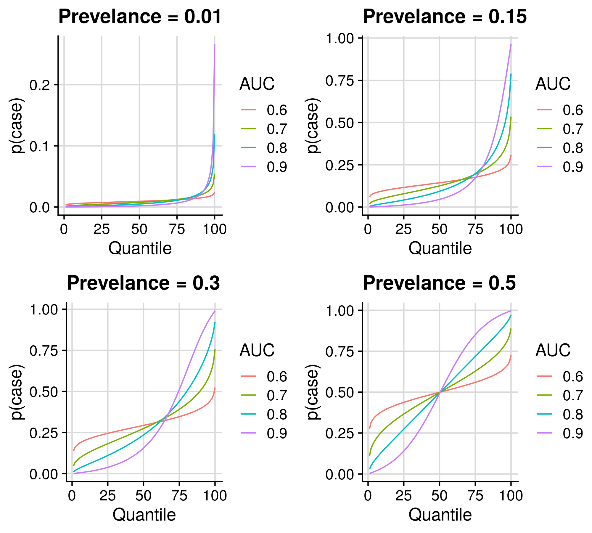
1.3 Demonstrate potential of polygenic scores

Here we will create a series of plots showing estimates on the absolute scale across PRS quantiles given a range of phenotype distribution and PRS AUC/R2.

---

1.3.1 Binary outcomes

Show code

# Thank you for Alex Gillet for her work developing this code.
ccprobs.f <- function(PRS_auc=0.641, prev=0.7463, n_quantile=20){
  
    # Convert AUC into cohen's d
    d <- sqrt(2)*qnorm(PRS_auc)
    
    # Set mean difference between cases and control polygenic scores
    mu_case <- d
    mu_control <- 0
    
    # Estimate mean and variance of polygenic scores across case and control
    varPRS <- prev*(1+(d^2) - (d*prev)^2) + (1-prev)*(1 - (d*prev)^2)
    E_PRS <- d*prev
    
    # Estimate polygenic score quantiles
    by_quant<-1/n_quantile
    p_quant <- seq(by_quant, 1-by_quant, by=by_quant)
    quant_vals_PRS <- rep(0, length(p_quant))
    quant_f_solve <- function(x, prev, d, pq){prev*pnorm(x-d) + (1-prev)*pnorm(x) - pq}
    for(i in 1:length(p_quant)){
        quant_vals_PRS[i] <- unlist(uniroot(quant_f_solve, prev=prev, d=d, pq= p_quant[i], interval=c(-2.5, 2.5), extendInt = "yes", tol=6e-12)$root)
    }
    
    # Create a table for output
    ul_qv_PRS <- matrix(0, ncol=2, nrow=n_quantile)
    ul_qv_PRS[1,1] <- -Inf
    ul_qv_PRS[2:n_quantile,1] <- quant_vals_PRS
    ul_qv_PRS[1:(n_quantile-1),2] <- quant_vals_PRS
    ul_qv_PRS[n_quantile,2] <- Inf
    
    ul_qv_PRS<-cbind(ul_qv_PRS, (ul_qv_PRS[,1:2]-E_PRS)/sqrt(varPRS))
    
    # Estimate case control proportion for each quantile
    prob_quantile_case <- pnorm(ul_qv_PRS[,2], mean = mu_case) - pnorm(ul_qv_PRS[,1], mean = mu_case)
    prob_quantile_control <- pnorm(ul_qv_PRS[,2], mean = mu_control) - pnorm(ul_qv_PRS[,1], mean = mu_control)
    p_case_quantile <- (prob_quantile_case*prev)/by_quant
    p_cont_quantile <- (prob_quantile_control*(1-prev))/by_quant
    
    # Estimate OR comparing each quantile to bottom quantile
    OR <- p_case_quantile/p_cont_quantile
    OR <- OR/OR[1]
    
    # Return output
    out <- cbind(ul_qv_PRS[,3:4],p_cont_quantile, p_case_quantile, OR)
    row.names(out) <- 1:n_quantile
    colnames(out) <- c("q_min", "q_max","p_control", "p_case", "OR")
    
    data.frame(out)
}

k<-as.character(c(0.01,0.15,0.3,0.5))
auc<-as.character(seq(0.6, 0.9, by=0.1))

library(ggplot2)
library(cowplot)

plot_list<-list()
plot_list_OR<-list()
res_all<-NULL
for(i in k){
  res_i<-NULL
  for(j in auc){
    res_i_j<-ccprobs.f(PRS_auc=as.numeric(j), prev=as.numeric(i), n_quantile=100)
    res_i_j$Quantile<-1:nrow(res_i_j)
    res_i_j$auc<-j
    res_i_j$k<-i
    res_i_j$OR<-res_i_j$p_case/as.numeric(i)
    res_i<-rbind(res_i, res_i_j)
  }
  
  res_all<-rbind(res_all, res_i)
  
  plot_list[[i]]<-ggplot(res_i, aes(x=Quantile, y=p_case, group=auc, colour=auc)) +
                    geom_line() +
                    labs(y="p(case)", title=paste0('Prevelance = ',i), colour='AUC')  +
                    theme_half_open() +
                    background_grid()

    plot_list_OR[[i]]<-ggplot(res_i, aes(x=Quantile, y=OR, group=auc, colour=auc)) +
                    geom_line() +
                    labs(y="OR", title=paste0('Prevelance = ',i), colour='AUC') +
                    theme_half_open() +
                    background_grid()
}

png(paste0('/scratch/users/k1806347/Analyses/AbsoluteRisk/Binary_sim.png'), units='px', res=300, width=2000, height=1800)
  plot_grid(plotlist=plot_list, ncol = 2)
dev.off()

png(paste0('/scratch/users/k1806347/Analyses/AbsoluteRisk/Binary_sim_OR.png'), units='px', res=300, width=2000, height=1800)
  plot_grid(plotlist=plot_list_OR, ncol = 2)
dev.off()

write.csv(res_all, '/scratch/users/k1806347/Analyses/AbsoluteRisk/Binary_sim.csv', row.names=F, quote=F)

Show results

Proportion of Cases within Polygenic Score Quantiles across AUC and prevelance

q_min	q_max	p_control	p_case	OR	Quantile	auc	k
-Inf	-2.326	0.996	0.004	0.366	1	0.6	0.01
-2.326	-2.054	0.996	0.004	0.433	2	0.6	0.01
-2.054	-1.881	0.995	0.005	0.467	3	0.6	0.01
-1.881	-1.751	0.995	0.005	0.493	4	0.6	0.01
-1.751	-1.645	0.995	0.005	0.514	5	0.6	0.01
-1.645	-1.555	0.995	0.005	0.532	6	0.6	0.01
-1.555	-1.476	0.995	0.005	0.548	7	0.6	0.01
-1.476	-1.405	0.994	0.006	0.563	8	0.6	0.01
-1.405	-1.341	0.994	0.006	0.577	9	0.6	0.01
-1.341	-1.281	0.994	0.006	0.589	10	0.6	0.01
-1.281	-1.226	0.994	0.006	0.602	11	0.6	0.01
-1.226	-1.175	0.994	0.006	0.613	12	0.6	0.01
-1.175	-1.126	0.994	0.006	0.624	13	0.6	0.01
-1.126	-1.080	0.994	0.006	0.635	14	0.6	0.01
-1.080	-1.036	0.994	0.006	0.645	15	0.6	0.01
-1.036	-0.994	0.993	0.007	0.655	16	0.6	0.01
-0.994	-0.954	0.993	0.007	0.664	17	0.6	0.01
-0.954	-0.915	0.993	0.007	0.674	18	0.6	0.01
-0.915	-0.878	0.993	0.007	0.683	19	0.6	0.01
-0.878	-0.842	0.993	0.007	0.692	20	0.6	0.01
-0.842	-0.806	0.993	0.007	0.701	21	0.6	0.01
-0.806	-0.772	0.993	0.007	0.710	22	0.6	0.01
-0.772	-0.739	0.993	0.007	0.718	23	0.6	0.01
-0.739	-0.706	0.993	0.007	0.727	24	0.6	0.01
-0.706	-0.675	0.993	0.007	0.735	25	0.6	0.01
-0.675	-0.643	0.993	0.007	0.743	26	0.6	0.01
-0.643	-0.613	0.992	0.008	0.752	27	0.6	0.01
-0.613	-0.583	0.992	0.008	0.760	28	0.6	0.01
-0.583	-0.553	0.992	0.008	0.768	29	0.6	0.01
-0.553	-0.524	0.992	0.008	0.776	30	0.6	0.01
-0.524	-0.496	0.992	0.008	0.784	31	0.6	0.01
-0.496	-0.468	0.992	0.008	0.792	32	0.6	0.01
-0.468	-0.440	0.992	0.008	0.800	33	0.6	0.01
-0.440	-0.413	0.992	0.008	0.808	34	0.6	0.01
-0.413	-0.385	0.992	0.008	0.815	35	0.6	0.01
-0.385	-0.359	0.992	0.008	0.823	36	0.6	0.01
-0.359	-0.332	0.992	0.008	0.831	37	0.6	0.01
-0.332	-0.306	0.992	0.008	0.839	38	0.6	0.01
-0.306	-0.279	0.992	0.008	0.847	39	0.6	0.01
-0.279	-0.253	0.991	0.009	0.855	40	0.6	0.01
-0.253	-0.228	0.991	0.009	0.863	41	0.6	0.01
-0.228	-0.202	0.991	0.009	0.871	42	0.6	0.01
-0.202	-0.176	0.991	0.009	0.879	43	0.6	0.01
-0.176	-0.151	0.991	0.009	0.887	44	0.6	0.01
-0.151	-0.126	0.991	0.009	0.895	45	0.6	0.01
-0.126	-0.101	0.991	0.009	0.903	46	0.6	0.01
-0.101	-0.075	0.991	0.009	0.911	47	0.6	0.01
-0.075	-0.050	0.991	0.009	0.919	48	0.6	0.01
-0.050	-0.025	0.991	0.009	0.927	49	0.6	0.01
-0.025	0.000	0.991	0.009	0.935	50	0.6	0.01
0.000	0.025	0.991	0.009	0.944	51	0.6	0.01
0.025	0.050	0.990	0.010	0.952	52	0.6	0.01
0.050	0.075	0.990	0.010	0.961	53	0.6	0.01
0.075	0.100	0.990	0.010	0.969	54	0.6	0.01
0.100	0.126	0.990	0.010	0.978	55	0.6	0.01
0.126	0.151	0.990	0.010	0.987	56	0.6	0.01
0.151	0.176	0.990	0.010	0.996	57	0.6	0.01
0.176	0.202	0.990	0.010	1.005	58	0.6	0.01
0.202	0.227	0.990	0.010	1.014	59	0.6	0.01
0.227	0.253	0.990	0.010	1.023	60	0.6	0.01
0.253	0.279	0.990	0.010	1.033	61	0.6	0.01
0.279	0.305	0.990	0.010	1.042	62	0.6	0.01
0.305	0.332	0.989	0.011	1.052	63	0.6	0.01
0.332	0.358	0.989	0.011	1.062	64	0.6	0.01
0.358	0.385	0.989	0.011	1.072	65	0.6	0.01
0.385	0.412	0.989	0.011	1.082	66	0.6	0.01
0.412	0.440	0.989	0.011	1.093	67	0.6	0.01
0.440	0.468	0.989	0.011	1.104	68	0.6	0.01
0.468	0.496	0.989	0.011	1.115	69	0.6	0.01
0.496	0.524	0.989	0.011	1.126	70	0.6	0.01
0.524	0.553	0.989	0.011	1.138	71	0.6	0.01
0.553	0.583	0.989	0.011	1.149	72	0.6	0.01
0.583	0.613	0.988	0.012	1.162	73	0.6	0.01
0.613	0.643	0.988	0.012	1.174	74	0.6	0.01
0.643	0.674	0.988	0.012	1.187	75	0.6	0.01
0.674	0.706	0.988	0.012	1.200	76	0.6	0.01
0.706	0.739	0.988	0.012	1.214	77	0.6	0.01
0.739	0.772	0.988	0.012	1.228	78	0.6	0.01
0.772	0.806	0.988	0.012	1.243	79	0.6	0.01
0.806	0.842	0.987	0.013	1.258	80	0.6	0.01
0.842	0.878	0.987	0.013	1.274	81	0.6	0.01
0.878	0.915	0.987	0.013	1.291	82	0.6	0.01
0.915	0.954	0.987	0.013	1.309	83	0.6	0.01
0.954	0.994	0.987	0.013	1.327	84	0.6	0.01
0.994	1.036	0.987	0.013	1.347	85	0.6	0.01
1.036	1.080	0.986	0.014	1.367	86	0.6	0.01
1.080	1.126	0.986	0.014	1.389	87	0.6	0.01
1.126	1.175	0.986	0.014	1.413	88	0.6	0.01
1.175	1.227	0.986	0.014	1.438	89	0.6	0.01
1.227	1.282	0.985	0.015	1.465	90	0.6	0.01
1.282	1.341	0.985	0.015	1.495	91	0.6	0.01
1.341	1.405	0.985	0.015	1.528	92	0.6	0.01
1.405	1.476	0.984	0.016	1.565	93	0.6	0.01
1.476	1.555	0.984	0.016	1.606	94	0.6	0.01
1.555	1.645	0.983	0.017	1.655	95	0.6	0.01
1.645	1.751	0.983	0.017	1.713	96	0.6	0.01
1.751	1.881	0.982	0.018	1.785	97	0.6	0.01
1.881	2.054	0.981	0.019	1.881	98	0.6	0.01
2.054	2.327	0.980	0.020	2.029	99	0.6	0.01
2.327	Inf	0.976	0.024	2.422	100	0.6	0.01
-Inf	-2.324	0.999	0.001	0.109	1	0.7	0.01
-2.324	-2.052	0.998	0.002	0.153	2	0.7	0.01
-2.052	-1.879	0.998	0.002	0.179	3	0.7	0.01
-1.879	-1.749	0.998	0.002	0.200	4	0.7	0.01
-1.749	-1.644	0.998	0.002	0.218	5	0.7	0.01
-1.644	-1.554	0.998	0.002	0.235	6	0.7	0.01
-1.554	-1.475	0.998	0.002	0.250	7	0.7	0.01
-1.475	-1.404	0.997	0.003	0.264	8	0.7	0.01
-1.404	-1.340	0.997	0.003	0.277	9	0.7	0.01
-1.340	-1.281	0.997	0.003	0.290	10	0.7	0.01
-1.281	-1.226	0.997	0.003	0.303	11	0.7	0.01
-1.226	-1.175	0.997	0.003	0.315	12	0.7	0.01
-1.175	-1.126	0.997	0.003	0.327	13	0.7	0.01
-1.126	-1.080	0.997	0.003	0.339	14	0.7	0.01
-1.080	-1.036	0.996	0.004	0.350	15	0.7	0.01
-1.036	-0.994	0.996	0.004	0.361	16	0.7	0.01
-0.994	-0.954	0.996	0.004	0.373	17	0.7	0.01
-0.954	-0.915	0.996	0.004	0.384	18	0.7	0.01
-0.915	-0.878	0.996	0.004	0.395	19	0.7	0.01
-0.878	-0.842	0.996	0.004	0.405	20	0.7	0.01
-0.842	-0.806	0.996	0.004	0.416	21	0.7	0.01
-0.806	-0.772	0.996	0.004	0.427	22	0.7	0.01
-0.772	-0.739	0.996	0.004	0.438	23	0.7	0.01
-0.739	-0.706	0.996	0.004	0.449	24	0.7	0.01
-0.706	-0.675	0.995	0.005	0.460	25	0.7	0.01
-0.675	-0.644	0.995	0.005	0.470	26	0.7	0.01
-0.644	-0.613	0.995	0.005	0.481	27	0.7	0.01
-0.613	-0.583	0.995	0.005	0.492	28	0.7	0.01
-0.583	-0.554	0.995	0.005	0.503	29	0.7	0.01
-0.554	-0.525	0.995	0.005	0.514	30	0.7	0.01
-0.525	-0.496	0.995	0.005	0.525	31	0.7	0.01
-0.496	-0.468	0.995	0.005	0.536	32	0.7	0.01
-0.468	-0.440	0.995	0.005	0.547	33	0.7	0.01
-0.440	-0.413	0.994	0.006	0.559	34	0.7	0.01
-0.413	-0.386	0.994	0.006	0.570	35	0.7	0.01
-0.386	-0.359	0.994	0.006	0.582	36	0.7	0.01
-0.359	-0.332	0.994	0.006	0.593	37	0.7	0.01
-0.332	-0.306	0.994	0.006	0.605	38	0.7	0.01
-0.306	-0.280	0.994	0.006	0.617	39	0.7	0.01
-0.280	-0.254	0.994	0.006	0.629	40	0.7	0.01
-0.254	-0.228	0.994	0.006	0.641	41	0.7	0.01
-0.228	-0.202	0.993	0.007	0.653	42	0.7	0.01
-0.202	-0.177	0.993	0.007	0.666	43	0.7	0.01
-0.177	-0.152	0.993	0.007	0.678	44	0.7	0.01
-0.152	-0.126	0.993	0.007	0.691	45	0.7	0.01
-0.126	-0.101	0.993	0.007	0.704	46	0.7	0.01
-0.101	-0.076	0.993	0.007	0.717	47	0.7	0.01
-0.076	-0.051	0.993	0.007	0.731	48	0.7	0.01
-0.051	-0.026	0.993	0.007	0.744	49	0.7	0.01
-0.026	-0.001	0.992	0.008	0.758	50	0.7	0.01
-0.001	0.024	0.992	0.008	0.772	51	0.7	0.01
0.024	0.050	0.992	0.008	0.787	52	0.7	0.01
0.050	0.075	0.992	0.008	0.801	53	0.7	0.01
0.075	0.100	0.992	0.008	0.816	54	0.7	0.01
0.100	0.125	0.992	0.008	0.832	55	0.7	0.01
0.125	0.150	0.992	0.008	0.847	56	0.7	0.01
0.150	0.176	0.991	0.009	0.863	57	0.7	0.01
0.176	0.201	0.991	0.009	0.880	58	0.7	0.01
0.201	0.227	0.991	0.009	0.896	59	0.7	0.01
0.227	0.253	0.991	0.009	0.914	60	0.7	0.01
0.253	0.279	0.991	0.009	0.931	61	0.7	0.01
0.279	0.305	0.991	0.009	0.949	62	0.7	0.01
0.305	0.331	0.990	0.010	0.968	63	0.7	0.01
0.331	0.358	0.990	0.010	0.987	64	0.7	0.01
0.358	0.385	0.990	0.010	1.007	65	0.7	0.01
0.385	0.412	0.990	0.010	1.027	66	0.7	0.01
0.412	0.439	0.990	0.010	1.048	67	0.7	0.01
0.439	0.467	0.989	0.011	1.069	68	0.7	0.01
0.467	0.495	0.989	0.011	1.091	69	0.7	0.01
0.495	0.524	0.989	0.011	1.114	70	0.7	0.01
0.524	0.553	0.989	0.011	1.138	71	0.7	0.01
0.553	0.582	0.988	0.012	1.163	72	0.7	0.01
0.582	0.612	0.988	0.012	1.189	73	0.7	0.01
0.612	0.643	0.988	0.012	1.215	74	0.7	0.01
0.643	0.674	0.988	0.012	1.243	75	0.7	0.01
0.674	0.706	0.987	0.013	1.272	76	0.7	0.01
0.706	0.738	0.987	0.013	1.303	77	0.7	0.01
0.738	0.772	0.987	0.013	1.335	78	0.7	0.01
0.772	0.806	0.986	0.014	1.368	79	0.7	0.01
0.806	0.841	0.986	0.014	1.403	80	0.7	0.01
0.841	0.878	0.986	0.014	1.441	81	0.7	0.01
0.878	0.915	0.985	0.015	1.480	82	0.7	0.01
0.915	0.954	0.985	0.015	1.522	83	0.7	0.01
0.954	0.994	0.984	0.016	1.567	84	0.7	0.01
0.994	1.036	0.984	0.016	1.615	85	0.7	0.01
1.036	1.080	0.983	0.017	1.666	86	0.7	0.01
1.080	1.126	0.983	0.017	1.722	87	0.7	0.01
1.126	1.175	0.982	0.018	1.783	88	0.7	0.01
1.175	1.227	0.982	0.018	1.849	89	0.7	0.01
1.227	1.282	0.981	0.019	1.922	90	0.7	0.01
1.282	1.341	0.980	0.020	2.004	91	0.7	0.01
1.341	1.405	0.979	0.021	2.097	92	0.7	0.01
1.405	1.476	0.978	0.022	2.202	93	0.7	0.01
1.476	1.556	0.977	0.023	2.325	94	0.7	0.01
1.556	1.646	0.975	0.025	2.472	95	0.7	0.01
1.646	1.752	0.973	0.027	2.654	96	0.7	0.01
1.752	1.882	0.971	0.029	2.889	97	0.7	0.01
1.882	2.056	0.968	0.032	3.219	98	0.7	0.01
2.056	2.330	0.962	0.038	3.760	99	0.7	0.01
2.330	Inf	0.945	0.055	5.458	100	0.7	0.01
-Inf	-2.318	1.000	0.000	0.022	1	0.8	0.01
-2.318	-2.047	1.000	0.000	0.038	2	0.8	0.01
-2.047	-1.875	1.000	0.000	0.048	3	0.8	0.01
-1.875	-1.746	0.999	0.001	0.058	4	0.8	0.01
-1.746	-1.641	0.999	0.001	0.066	5	0.8	0.01
-1.641	-1.551	0.999	0.001	0.075	6	0.8	0.01
-1.551	-1.472	0.999	0.001	0.082	7	0.8	0.01
-1.472	-1.402	0.999	0.001	0.090	8	0.8	0.01
-1.402	-1.338	0.999	0.001	0.098	9	0.8	0.01
-1.338	-1.279	0.999	0.001	0.105	10	0.8	0.01
-1.279	-1.224	0.999	0.001	0.112	11	0.8	0.01
-1.224	-1.173	0.999	0.001	0.120	12	0.8	0.01
-1.173	-1.125	0.999	0.001	0.127	13	0.8	0.01
-1.125	-1.079	0.999	0.001	0.135	14	0.8	0.01
-1.079	-1.035	0.999	0.001	0.142	15	0.8	0.01
-1.035	-0.993	0.999	0.001	0.149	16	0.8	0.01
-0.993	-0.953	0.998	0.002	0.157	17	0.8	0.01
-0.953	-0.915	0.998	0.002	0.164	18	0.8	0.01
-0.915	-0.877	0.998	0.002	0.172	19	0.8	0.01
-0.877	-0.841	0.998	0.002	0.180	20	0.8	0.01
-0.841	-0.806	0.998	0.002	0.188	21	0.8	0.01
-0.806	-0.772	0.998	0.002	0.196	22	0.8	0.01
-0.772	-0.739	0.998	0.002	0.204	23	0.8	0.01
-0.739	-0.706	0.998	0.002	0.212	24	0.8	0.01
-0.706	-0.675	0.998	0.002	0.220	25	0.8	0.01
-0.675	-0.644	0.998	0.002	0.228	26	0.8	0.01
-0.644	-0.613	0.998	0.002	0.237	27	0.8	0.01
-0.613	-0.583	0.998	0.002	0.246	28	0.8	0.01
-0.583	-0.554	0.997	0.003	0.255	29	0.8	0.01
-0.554	-0.525	0.997	0.003	0.264	30	0.8	0.01
-0.525	-0.497	0.997	0.003	0.273	31	0.8	0.01
-0.497	-0.469	0.997	0.003	0.282	32	0.8	0.01
-0.469	-0.441	0.997	0.003	0.292	33	0.8	0.01
-0.441	-0.414	0.997	0.003	0.301	34	0.8	0.01
-0.414	-0.387	0.997	0.003	0.311	35	0.8	0.01
-0.387	-0.360	0.997	0.003	0.322	36	0.8	0.01
-0.360	-0.333	0.997	0.003	0.332	37	0.8	0.01
-0.333	-0.307	0.997	0.003	0.343	38	0.8	0.01
-0.307	-0.281	0.996	0.004	0.353	39	0.8	0.01
-0.281	-0.255	0.996	0.004	0.365	40	0.8	0.01
-0.255	-0.229	0.996	0.004	0.376	41	0.8	0.01
-0.229	-0.204	0.996	0.004	0.388	42	0.8	0.01
-0.204	-0.178	0.996	0.004	0.400	43	0.8	0.01
-0.178	-0.153	0.996	0.004	0.412	44	0.8	0.01
-0.153	-0.128	0.996	0.004	0.425	45	0.8	0.01
-0.128	-0.102	0.996	0.004	0.438	46	0.8	0.01
-0.102	-0.077	0.995	0.005	0.451	47	0.8	0.01
-0.077	-0.052	0.995	0.005	0.465	48	0.8	0.01
-0.052	-0.027	0.995	0.005	0.479	49	0.8	0.01
-0.027	-0.002	0.995	0.005	0.493	50	0.8	0.01
-0.002	0.023	0.995	0.005	0.508	51	0.8	0.01
0.023	0.048	0.995	0.005	0.524	52	0.8	0.01
0.048	0.073	0.995	0.005	0.539	53	0.8	0.01
0.073	0.098	0.994	0.006	0.556	54	0.8	0.01
0.098	0.123	0.994	0.006	0.573	55	0.8	0.01
0.123	0.148	0.994	0.006	0.590	56	0.8	0.01
0.148	0.174	0.994	0.006	0.608	57	0.8	0.01
0.174	0.199	0.994	0.006	0.627	58	0.8	0.01
0.199	0.225	0.994	0.006	0.646	59	0.8	0.01
0.225	0.251	0.993	0.007	0.667	60	0.8	0.01
0.251	0.277	0.993	0.007	0.687	61	0.8	0.01
0.277	0.303	0.993	0.007	0.709	62	0.8	0.01
0.303	0.329	0.993	0.007	0.732	63	0.8	0.01
0.329	0.356	0.992	0.008	0.755	64	0.8	0.01
0.356	0.383	0.992	0.008	0.779	65	0.8	0.01
0.383	0.410	0.992	0.008	0.805	66	0.8	0.01
0.410	0.437	0.992	0.008	0.831	67	0.8	0.01
0.437	0.465	0.991	0.009	0.859	68	0.8	0.01
0.465	0.493	0.991	0.009	0.888	69	0.8	0.01
0.493	0.522	0.991	0.009	0.918	70	0.8	0.01
0.522	0.551	0.990	0.010	0.950	71	0.8	0.01
0.551	0.580	0.990	0.010	0.984	72	0.8	0.01
0.580	0.610	0.990	0.010	1.019	73	0.8	0.01
0.610	0.641	0.989	0.011	1.057	74	0.8	0.01
0.641	0.672	0.989	0.011	1.096	75	0.8	0.01
0.672	0.704	0.989	0.011	1.138	76	0.8	0.01
0.704	0.736	0.988	0.012	1.182	77	0.8	0.01
0.736	0.770	0.988	0.012	1.229	78	0.8	0.01
0.770	0.804	0.987	0.013	1.279	79	0.8	0.01
0.804	0.839	0.987	0.013	1.333	80	0.8	0.01
0.839	0.876	0.986	0.014	1.391	81	0.8	0.01
0.876	0.913	0.985	0.015	1.453	82	0.8	0.01
0.913	0.952	0.985	0.015	1.520	83	0.8	0.01
0.952	0.993	0.984	0.016	1.593	84	0.8	0.01
0.993	1.035	0.983	0.017	1.672	85	0.8	0.01
1.035	1.079	0.982	0.018	1.759	86	0.8	0.01
1.079	1.125	0.981	0.019	1.855	87	0.8	0.01
1.125	1.174	0.980	0.020	1.962	88	0.8	0.01
1.174	1.226	0.979	0.021	2.082	89	0.8	0.01
1.226	1.281	0.978	0.022	2.217	90	0.8	0.01
1.281	1.341	0.976	0.024	2.371	91	0.8	0.01
1.341	1.406	0.975	0.025	2.549	92	0.8	0.01
1.406	1.477	0.972	0.028	2.760	93	0.8	0.01
1.477	1.557	0.970	0.030	3.013	94	0.8	0.01
1.557	1.648	0.967	0.033	3.326	95	0.8	0.01
1.648	1.755	0.963	0.037	3.728	96	0.8	0.01
1.755	1.887	0.957	0.043	4.275	97	0.8	0.01
1.887	2.063	0.949	0.051	5.086	98	0.8	0.01
2.063	2.342	0.935	0.065	6.523	99	0.8	0.01
2.342	Inf	0.881	0.119	11.908	100	0.8	0.01
-Inf	-2.304	1.000	0.000	0.002	1	0.9	0.01
-2.304	-2.035	1.000	0.000	0.004	2	0.9	0.01
-2.035	-1.864	1.000	0.000	0.006	3	0.9	0.01
-1.864	-1.736	1.000	0.000	0.007	4	0.9	0.01
-1.736	-1.632	1.000	0.000	0.009	5	0.9	0.01
-1.632	-1.543	1.000	0.000	0.011	6	0.9	0.01
-1.543	-1.465	1.000	0.000	0.013	7	0.9	0.01
-1.465	-1.395	1.000	0.000	0.015	8	0.9	0.01
-1.395	-1.332	1.000	0.000	0.016	9	0.9	0.01
-1.332	-1.273	1.000	0.000	0.018	10	0.9	0.01
-1.273	-1.219	1.000	0.000	0.020	11	0.9	0.01
-1.219	-1.168	1.000	0.000	0.022	12	0.9	0.01
-1.168	-1.120	1.000	0.000	0.025	13	0.9	0.01
-1.120	-1.075	1.000	0.000	0.027	14	0.9	0.01
-1.075	-1.032	1.000	0.000	0.029	15	0.9	0.01
-1.032	-0.990	1.000	0.000	0.031	16	0.9	0.01
-0.990	-0.950	1.000	0.000	0.034	17	0.9	0.01
-0.950	-0.912	1.000	0.000	0.036	18	0.9	0.01
-0.912	-0.875	1.000	0.000	0.039	19	0.9	0.01
-0.875	-0.839	1.000	0.000	0.042	20	0.9	0.01
-0.839	-0.804	1.000	0.000	0.044	21	0.9	0.01
-0.804	-0.771	1.000	0.000	0.047	22	0.9	0.01
-0.771	-0.738	0.999	0.001	0.050	23	0.9	0.01
-0.738	-0.705	0.999	0.001	0.053	24	0.9	0.01
-0.705	-0.674	0.999	0.001	0.057	25	0.9	0.01
-0.674	-0.643	0.999	0.001	0.060	26	0.9	0.01
-0.643	-0.613	0.999	0.001	0.064	27	0.9	0.01
-0.613	-0.583	0.999	0.001	0.067	28	0.9	0.01
-0.583	-0.554	0.999	0.001	0.071	29	0.9	0.01
-0.554	-0.526	0.999	0.001	0.075	30	0.9	0.01
-0.526	-0.497	0.999	0.001	0.079	31	0.9	0.01
-0.497	-0.470	0.999	0.001	0.083	32	0.9	0.01
-0.470	-0.442	0.999	0.001	0.087	33	0.9	0.01
-0.442	-0.415	0.999	0.001	0.092	34	0.9	0.01
-0.415	-0.388	0.999	0.001	0.096	35	0.9	0.01
-0.388	-0.361	0.999	0.001	0.101	36	0.9	0.01
-0.361	-0.335	0.999	0.001	0.106	37	0.9	0.01
-0.335	-0.309	0.999	0.001	0.112	38	0.9	0.01
-0.309	-0.283	0.999	0.001	0.117	39	0.9	0.01
-0.283	-0.257	0.999	0.001	0.123	40	0.9	0.01
-0.257	-0.232	0.999	0.001	0.129	41	0.9	0.01
-0.232	-0.206	0.999	0.001	0.135	42	0.9	0.01
-0.206	-0.181	0.999	0.001	0.141	43	0.9	0.01
-0.181	-0.156	0.999	0.001	0.148	44	0.9	0.01
-0.156	-0.131	0.998	0.002	0.155	45	0.9	0.01
-0.131	-0.106	0.998	0.002	0.162	46	0.9	0.01
-0.106	-0.081	0.998	0.002	0.170	47	0.9	0.01
-0.081	-0.056	0.998	0.002	0.178	48	0.9	0.01
-0.056	-0.031	0.998	0.002	0.186	49	0.9	0.01
-0.031	-0.006	0.998	0.002	0.195	50	0.9	0.01
-0.006	0.019	0.998	0.002	0.204	51	0.9	0.01
0.019	0.043	0.998	0.002	0.213	52	0.9	0.01
0.043	0.068	0.998	0.002	0.223	53	0.9	0.01
0.068	0.093	0.998	0.002	0.234	54	0.9	0.01
0.093	0.118	0.998	0.002	0.245	55	0.9	0.01
0.118	0.144	0.997	0.003	0.256	56	0.9	0.01
0.144	0.169	0.997	0.003	0.269	57	0.9	0.01
0.169	0.194	0.997	0.003	0.281	58	0.9	0.01
0.194	0.220	0.997	0.003	0.295	59	0.9	0.01
0.220	0.245	0.997	0.003	0.309	60	0.9	0.01
0.245	0.271	0.997	0.003	0.324	61	0.9	0.01
0.271	0.297	0.997	0.003	0.340	62	0.9	0.01
0.297	0.323	0.996	0.004	0.357	63	0.9	0.01
0.323	0.350	0.996	0.004	0.374	64	0.9	0.01
0.350	0.377	0.996	0.004	0.393	65	0.9	0.01
0.377	0.404	0.996	0.004	0.413	66	0.9	0.01
0.404	0.431	0.996	0.004	0.434	67	0.9	0.01
0.431	0.459	0.995	0.005	0.456	68	0.9	0.01
0.459	0.487	0.995	0.005	0.480	69	0.9	0.01
0.487	0.515	0.995	0.005	0.506	70	0.9	0.01
0.515	0.544	0.995	0.005	0.533	71	0.9	0.01
0.544	0.574	0.994	0.006	0.562	72	0.9	0.01
0.574	0.604	0.994	0.006	0.594	73	0.9	0.01
0.604	0.634	0.994	0.006	0.628	74	0.9	0.01
0.634	0.665	0.993	0.007	0.664	75	0.9	0.01
0.665	0.697	0.993	0.007	0.703	76	0.9	0.01
0.697	0.730	0.993	0.007	0.746	77	0.9	0.01
0.730	0.763	0.992	0.008	0.793	78	0.9	0.01
0.763	0.798	0.992	0.008	0.843	79	0.9	0.01
0.798	0.833	0.991	0.009	0.898	80	0.9	0.01
0.833	0.869	0.990	0.010	0.959	81	0.9	0.01
0.869	0.907	0.990	0.010	1.026	82	0.9	0.01
0.907	0.946	0.989	0.011	1.101	83	0.9	0.01
0.946	0.987	0.988	0.012	1.183	84	0.9	0.01
0.987	1.029	0.987	0.013	1.276	85	0.9	0.01
1.029	1.073	0.986	0.014	1.381	86	0.9	0.01
1.073	1.120	0.985	0.015	1.499	87	0.9	0.01
1.120	1.169	0.984	0.016	1.635	88	0.9	0.01
1.169	1.222	0.982	0.018	1.793	89	0.9	0.01
1.222	1.278	0.980	0.020	1.977	90	0.9	0.01
1.278	1.338	0.978	0.022	2.196	91	0.9	0.01
1.338	1.404	0.975	0.025	2.459	92	0.9	0.01
1.404	1.476	0.972	0.028	2.783	93	0.9	0.01
1.476	1.558	0.968	0.032	3.193	94	0.9	0.01
1.558	1.651	0.963	0.037	3.728	95	0.9	0.01
1.651	1.761	0.955	0.045	4.459	96	0.9	0.01
1.761	1.898	0.945	0.055	5.529	97	0.9	0.01
1.898	2.082	0.927	0.073	7.271	98	0.9	0.01
2.082	2.380	0.892	0.108	10.768	99	0.9	0.01
2.380	Inf	0.734	0.266	26.623	100	0.9	0.01
-Inf	-2.324	0.939	0.061	0.406	1	0.6	0.15
-2.324	-2.052	0.929	0.071	0.476	2	0.6	0.15
-2.052	-1.879	0.923	0.077	0.512	3	0.6	0.15
-1.879	-1.749	0.919	0.081	0.538	4	0.6	0.15
-1.749	-1.644	0.916	0.084	0.559	5	0.6	0.15
-1.644	-1.554	0.913	0.087	0.577	6	0.6	0.15
-1.554	-1.475	0.911	0.089	0.593	7	0.6	0.15
-1.475	-1.404	0.909	0.091	0.608	8	0.6	0.15
-1.404	-1.340	0.907	0.093	0.621	9	0.6	0.15
-1.340	-1.281	0.905	0.095	0.634	10	0.6	0.15
-1.281	-1.226	0.903	0.097	0.646	11	0.6	0.15
-1.226	-1.175	0.901	0.099	0.657	12	0.6	0.15
-1.175	-1.126	0.900	0.100	0.668	13	0.6	0.15
-1.126	-1.080	0.898	0.102	0.678	14	0.6	0.15
-1.080	-1.036	0.897	0.103	0.688	15	0.6	0.15
-1.036	-0.994	0.895	0.105	0.698	16	0.6	0.15
-0.994	-0.954	0.894	0.106	0.707	17	0.6	0.15
-0.954	-0.915	0.893	0.107	0.716	18	0.6	0.15
-0.915	-0.878	0.891	0.109	0.725	19	0.6	0.15
-0.878	-0.842	0.890	0.110	0.734	20	0.6	0.15
-0.842	-0.807	0.889	0.111	0.742	21	0.6	0.15
-0.807	-0.772	0.887	0.113	0.751	22	0.6	0.15
-0.772	-0.739	0.886	0.114	0.759	23	0.6	0.15
-0.739	-0.707	0.885	0.115	0.767	24	0.6	0.15
-0.707	-0.675	0.884	0.116	0.775	25	0.6	0.15
-0.675	-0.644	0.883	0.117	0.782	26	0.6	0.15
-0.644	-0.613	0.881	0.119	0.790	27	0.6	0.15
-0.613	-0.583	0.880	0.120	0.798	28	0.6	0.15
-0.583	-0.554	0.879	0.121	0.805	29	0.6	0.15
-0.554	-0.525	0.878	0.122	0.813	30	0.6	0.15
-0.525	-0.496	0.877	0.123	0.820	31	0.6	0.15
-0.496	-0.468	0.876	0.124	0.828	32	0.6	0.15
-0.468	-0.440	0.875	0.125	0.835	33	0.6	0.15
-0.440	-0.413	0.874	0.126	0.842	34	0.6	0.15
-0.413	-0.386	0.873	0.127	0.850	35	0.6	0.15
-0.386	-0.359	0.871	0.129	0.857	36	0.6	0.15
-0.359	-0.332	0.870	0.130	0.864	37	0.6	0.15
-0.332	-0.306	0.869	0.131	0.871	38	0.6	0.15
-0.306	-0.280	0.868	0.132	0.879	39	0.6	0.15
-0.280	-0.254	0.867	0.133	0.886	40	0.6	0.15
-0.254	-0.228	0.866	0.134	0.893	41	0.6	0.15
-0.228	-0.203	0.865	0.135	0.900	42	0.6	0.15
-0.203	-0.177	0.864	0.136	0.907	43	0.6	0.15
-0.177	-0.152	0.863	0.137	0.915	44	0.6	0.15
-0.152	-0.126	0.862	0.138	0.922	45	0.6	0.15
-0.126	-0.101	0.861	0.139	0.929	46	0.6	0.15
-0.101	-0.076	0.860	0.140	0.936	47	0.6	0.15
-0.076	-0.051	0.858	0.142	0.944	48	0.6	0.15
-0.051	-0.026	0.857	0.143	0.951	49	0.6	0.15
-0.026	-0.001	0.856	0.144	0.958	50	0.6	0.15
-0.001	0.024	0.855	0.145	0.966	51	0.6	0.15
0.024	0.049	0.854	0.146	0.973	52	0.6	0.15
0.049	0.075	0.853	0.147	0.981	53	0.6	0.15
0.075	0.100	0.852	0.148	0.989	54	0.6	0.15
0.100	0.125	0.851	0.149	0.996	55	0.6	0.15
0.125	0.150	0.849	0.151	1.004	56	0.6	0.15
0.150	0.176	0.848	0.152	1.012	57	0.6	0.15
0.176	0.201	0.847	0.153	1.020	58	0.6	0.15
0.201	0.227	0.846	0.154	1.028	59	0.6	0.15
0.227	0.253	0.845	0.155	1.036	60	0.6	0.15
0.253	0.279	0.843	0.157	1.044	61	0.6	0.15
0.279	0.305	0.842	0.158	1.052	62	0.6	0.15
0.305	0.331	0.841	0.159	1.061	63	0.6	0.15
0.331	0.358	0.840	0.160	1.069	64	0.6	0.15
0.358	0.385	0.838	0.162	1.078	65	0.6	0.15
0.385	0.412	0.837	0.163	1.087	66	0.6	0.15
0.412	0.439	0.836	0.164	1.096	67	0.6	0.15
0.439	0.467	0.834	0.166	1.105	68	0.6	0.15
0.467	0.495	0.833	0.167	1.115	69	0.6	0.15
0.495	0.524	0.831	0.169	1.124	70	0.6	0.15
0.524	0.553	0.830	0.170	1.134	71	0.6	0.15
0.553	0.582	0.828	0.172	1.144	72	0.6	0.15
0.582	0.612	0.827	0.173	1.154	73	0.6	0.15
0.612	0.643	0.825	0.175	1.165	74	0.6	0.15
0.643	0.674	0.824	0.176	1.175	75	0.6	0.15
0.674	0.706	0.822	0.178	1.186	76	0.6	0.15
0.706	0.739	0.820	0.180	1.198	77	0.6	0.15
0.739	0.772	0.819	0.181	1.209	78	0.6	0.15
0.772	0.806	0.817	0.183	1.222	79	0.6	0.15
0.806	0.841	0.815	0.185	1.234	80	0.6	0.15
0.841	0.878	0.813	0.187	1.247	81	0.6	0.15
0.878	0.915	0.811	0.189	1.261	82	0.6	0.15
0.915	0.954	0.809	0.191	1.275	83	0.6	0.15
0.954	0.994	0.807	0.193	1.290	84	0.6	0.15
0.994	1.036	0.804	0.196	1.305	85	0.6	0.15
1.036	1.080	0.802	0.198	1.322	86	0.6	0.15
1.080	1.127	0.799	0.201	1.339	87	0.6	0.15
1.127	1.175	0.796	0.204	1.357	88	0.6	0.15
1.175	1.227	0.793	0.207	1.377	89	0.6	0.15
1.227	1.282	0.790	0.210	1.398	90	0.6	0.15
1.282	1.341	0.787	0.213	1.421	91	0.6	0.15
1.341	1.406	0.783	0.217	1.446	92	0.6	0.15
1.406	1.477	0.779	0.221	1.474	93	0.6	0.15
1.477	1.556	0.774	0.226	1.505	94	0.6	0.15
1.556	1.646	0.769	0.231	1.541	95	0.6	0.15
1.646	1.752	0.762	0.238	1.583	96	0.6	0.15
1.752	1.883	0.755	0.245	1.635	97	0.6	0.15
1.883	2.056	0.745	0.255	1.703	98	0.6	0.15
2.056	2.329	0.730	0.270	1.803	99	0.6	0.15
2.329	Inf	0.693	0.307	2.048	100	0.6	0.15
-Inf	-2.304	0.981	0.019	0.129	1	0.7	0.15
-2.304	-2.037	0.973	0.027	0.181	2	0.7	0.15
-2.037	-1.867	0.968	0.032	0.211	3	0.7	0.15
-1.867	-1.739	0.965	0.035	0.235	4	0.7	0.15
-1.739	-1.635	0.962	0.038	0.256	5	0.7	0.15
-1.635	-1.546	0.959	0.041	0.275	6	0.7	0.15
-1.546	-1.469	0.956	0.044	0.292	7	0.7	0.15
-1.469	-1.399	0.954	0.046	0.308	8	0.7	0.15
-1.399	-1.336	0.951	0.049	0.324	9	0.7	0.15
-1.336	-1.277	0.949	0.051	0.338	10	0.7	0.15
-1.277	-1.223	0.947	0.053	0.352	11	0.7	0.15
-1.223	-1.172	0.945	0.055	0.366	12	0.7	0.15
-1.172	-1.124	0.943	0.057	0.379	13	0.7	0.15
-1.124	-1.079	0.941	0.059	0.392	14	0.7	0.15
-1.079	-1.035	0.939	0.061	0.405	15	0.7	0.15
-1.035	-0.994	0.937	0.063	0.418	16	0.7	0.15
-0.994	-0.954	0.935	0.065	0.430	17	0.7	0.15
-0.954	-0.915	0.934	0.066	0.442	18	0.7	0.15
-0.915	-0.878	0.932	0.068	0.454	19	0.7	0.15
-0.878	-0.842	0.930	0.070	0.466	20	0.7	0.15
-0.842	-0.808	0.928	0.072	0.478	21	0.7	0.15
-0.808	-0.774	0.926	0.074	0.490	22	0.7	0.15
-0.774	-0.741	0.925	0.075	0.502	23	0.7	0.15
-0.741	-0.708	0.923	0.077	0.514	24	0.7	0.15
-0.708	-0.677	0.921	0.079	0.526	25	0.7	0.15
-0.677	-0.646	0.919	0.081	0.537	26	0.7	0.15
-0.646	-0.616	0.918	0.082	0.549	27	0.7	0.15
-0.616	-0.586	0.916	0.084	0.561	28	0.7	0.15
-0.586	-0.557	0.914	0.086	0.572	29	0.7	0.15
-0.557	-0.528	0.912	0.088	0.584	30	0.7	0.15
-0.528	-0.500	0.911	0.089	0.596	31	0.7	0.15
-0.500	-0.472	0.909	0.091	0.608	32	0.7	0.15
-0.472	-0.444	0.907	0.093	0.620	33	0.7	0.15
-0.444	-0.417	0.905	0.095	0.632	34	0.7	0.15
-0.417	-0.390	0.903	0.097	0.644	35	0.7	0.15
-0.390	-0.363	0.902	0.098	0.656	36	0.7	0.15
-0.363	-0.337	0.900	0.100	0.668	37	0.7	0.15
-0.337	-0.310	0.898	0.102	0.680	38	0.7	0.15
-0.310	-0.284	0.896	0.104	0.692	39	0.7	0.15
-0.284	-0.258	0.894	0.106	0.705	40	0.7	0.15
-0.258	-0.233	0.892	0.108	0.717	41	0.7	0.15
-0.233	-0.207	0.890	0.110	0.730	42	0.7	0.15
-0.207	-0.182	0.889	0.111	0.743	43	0.7	0.15
-0.182	-0.156	0.887	0.113	0.756	44	0.7	0.15
-0.156	-0.131	0.885	0.115	0.769	45	0.7	0.15
-0.131	-0.106	0.883	0.117	0.782	46	0.7	0.15
-0.106	-0.081	0.881	0.119	0.796	47	0.7	0.15
-0.081	-0.056	0.879	0.121	0.809	48	0.7	0.15
-0.056	-0.031	0.877	0.123	0.823	49	0.7	0.15
-0.031	-0.006	0.874	0.126	0.837	50	0.7	0.15
-0.006	0.019	0.872	0.128	0.851	51	0.7	0.15
0.019	0.044	0.870	0.130	0.865	52	0.7	0.15
0.044	0.070	0.868	0.132	0.880	53	0.7	0.15
0.070	0.095	0.866	0.134	0.895	54	0.7	0.15
0.095	0.120	0.864	0.136	0.910	55	0.7	0.15
0.120	0.145	0.861	0.139	0.925	56	0.7	0.15
0.145	0.171	0.859	0.141	0.941	57	0.7	0.15
0.171	0.196	0.856	0.144	0.957	58	0.7	0.15
0.196	0.222	0.854	0.146	0.973	59	0.7	0.15
0.222	0.248	0.852	0.148	0.990	60	0.7	0.15
0.248	0.274	0.849	0.151	1.006	61	0.7	0.15
0.274	0.300	0.846	0.154	1.024	62	0.7	0.15
0.300	0.326	0.844	0.156	1.041	63	0.7	0.15
0.326	0.353	0.841	0.159	1.059	64	0.7	0.15
0.353	0.380	0.838	0.162	1.078	65	0.7	0.15
0.380	0.407	0.835	0.165	1.097	66	0.7	0.15
0.407	0.435	0.833	0.167	1.116	67	0.7	0.15
0.435	0.463	0.830	0.170	1.136	68	0.7	0.15
0.463	0.491	0.827	0.173	1.156	69	0.7	0.15
0.491	0.520	0.823	0.177	1.178	70	0.7	0.15
0.520	0.549	0.820	0.180	1.199	71	0.7	0.15
0.549	0.579	0.817	0.183	1.222	72	0.7	0.15
0.579	0.609	0.813	0.187	1.245	73	0.7	0.15
0.609	0.639	0.810	0.190	1.268	74	0.7	0.15
0.639	0.671	0.806	0.194	1.293	75	0.7	0.15
0.671	0.703	0.802	0.198	1.319	76	0.7	0.15
0.703	0.736	0.798	0.202	1.345	77	0.7	0.15
0.736	0.769	0.794	0.206	1.373	78	0.7	0.15
0.769	0.804	0.790	0.210	1.401	79	0.7	0.15
0.804	0.839	0.785	0.215	1.431	80	0.7	0.15
0.839	0.876	0.781	0.219	1.463	81	0.7	0.15
0.876	0.914	0.776	0.224	1.496	82	0.7	0.15
0.914	0.953	0.770	0.230	1.530	83	0.7	0.15
0.953	0.994	0.765	0.235	1.567	84	0.7	0.15
0.994	1.036	0.759	0.241	1.605	85	0.7	0.15
1.036	1.081	0.753	0.247	1.646	86	0.7	0.15
1.081	1.127	0.747	0.253	1.690	87	0.7	0.15
1.127	1.177	0.740	0.260	1.737	88	0.7	0.15
1.177	1.229	0.732	0.268	1.787	89	0.7	0.15
1.229	1.285	0.724	0.276	1.842	90	0.7	0.15
1.285	1.345	0.715	0.285	1.902	91	0.7	0.15
1.345	1.410	0.705	0.295	1.968	92	0.7	0.15
1.410	1.482	0.694	0.306	2.041	93	0.7	0.15
1.482	1.563	0.681	0.319	2.125	94	0.7	0.15
1.563	1.655	0.667	0.333	2.221	95	0.7	0.15
1.655	1.763	0.650	0.350	2.336	96	0.7	0.15
1.763	1.896	0.628	0.372	2.477	97	0.7	0.15
1.896	2.073	0.601	0.399	2.662	98	0.7	0.15
2.073	2.352	0.560	0.440	2.935	99	0.7	0.15
2.352	Inf	0.465	0.535	3.568	100	0.7	0.15
-Inf	-2.250	0.996	0.004	0.027	1	0.8	0.15
-2.250	-1.994	0.993	0.007	0.047	2	0.8	0.15
-1.994	-1.831	0.991	0.009	0.060	3	0.8	0.15
-1.831	-1.708	0.989	0.011	0.072	4	0.8	0.15
-1.708	-1.608	0.988	0.012	0.083	5	0.8	0.15
-1.608	-1.523	0.986	0.014	0.093	6	0.8	0.15
-1.523	-1.448	0.984	0.016	0.103	7	0.8	0.15
-1.448	-1.381	0.983	0.017	0.113	8	0.8	0.15
-1.381	-1.320	0.982	0.018	0.123	9	0.8	0.15
-1.320	-1.264	0.980	0.020	0.132	10	0.8	0.15
-1.264	-1.211	0.979	0.021	0.142	11	0.8	0.15
-1.211	-1.162	0.977	0.023	0.151	12	0.8	0.15
-1.162	-1.116	0.976	0.024	0.160	13	0.8	0.15
-1.116	-1.072	0.975	0.025	0.170	14	0.8	0.15
-1.072	-1.030	0.973	0.027	0.179	15	0.8	0.15
-1.030	-0.989	0.972	0.028	0.189	16	0.8	0.15
-0.989	-0.951	0.970	0.030	0.198	17	0.8	0.15
-0.951	-0.914	0.969	0.031	0.208	18	0.8	0.15
-0.914	-0.878	0.967	0.033	0.218	19	0.8	0.15
-0.878	-0.843	0.966	0.034	0.228	20	0.8	0.15
-0.843	-0.809	0.964	0.036	0.238	21	0.8	0.15
-0.809	-0.776	0.963	0.037	0.248	22	0.8	0.15
-0.776	-0.744	0.961	0.039	0.258	23	0.8	0.15
-0.744	-0.712	0.960	0.040	0.268	24	0.8	0.15
-0.712	-0.681	0.958	0.042	0.279	25	0.8	0.15
-0.681	-0.651	0.957	0.043	0.290	26	0.8	0.15
-0.651	-0.622	0.955	0.045	0.300	27	0.8	0.15
-0.622	-0.593	0.953	0.047	0.311	28	0.8	0.15
-0.593	-0.564	0.952	0.048	0.323	29	0.8	0.15
-0.564	-0.536	0.950	0.050	0.334	30	0.8	0.15
-0.536	-0.508	0.948	0.052	0.346	31	0.8	0.15
-0.508	-0.481	0.946	0.054	0.358	32	0.8	0.15
-0.481	-0.454	0.945	0.055	0.370	33	0.8	0.15
-0.454	-0.427	0.943	0.057	0.382	34	0.8	0.15
-0.427	-0.401	0.941	0.059	0.395	35	0.8	0.15
-0.401	-0.374	0.939	0.061	0.408	36	0.8	0.15
-0.374	-0.348	0.937	0.063	0.421	37	0.8	0.15
-0.348	-0.322	0.935	0.065	0.434	38	0.8	0.15
-0.322	-0.297	0.933	0.067	0.448	39	0.8	0.15
-0.297	-0.271	0.931	0.069	0.462	40	0.8	0.15
-0.271	-0.246	0.929	0.071	0.476	41	0.8	0.15
-0.246	-0.221	0.926	0.074	0.491	42	0.8	0.15
-0.221	-0.196	0.924	0.076	0.506	43	0.8	0.15
-0.196	-0.171	0.922	0.078	0.521	44	0.8	0.15
-0.171	-0.146	0.919	0.081	0.537	45	0.8	0.15
-0.146	-0.121	0.917	0.083	0.553	46	0.8	0.15
-0.121	-0.096	0.915	0.085	0.570	47	0.8	0.15
-0.096	-0.071	0.912	0.088	0.587	48	0.8	0.15
-0.071	-0.046	0.909	0.091	0.604	49	0.8	0.15
-0.046	-0.021	0.907	0.093	0.622	50	0.8	0.15
-0.021	0.003	0.904	0.096	0.640	51	0.8	0.15
0.003	0.028	0.901	0.099	0.659	52	0.8	0.15
0.028	0.053	0.898	0.102	0.679	53	0.8	0.15
0.053	0.078	0.895	0.105	0.699	54	0.8	0.15
0.078	0.104	0.892	0.108	0.719	55	0.8	0.15
0.104	0.129	0.889	0.111	0.740	56	0.8	0.15
0.129	0.154	0.886	0.114	0.762	57	0.8	0.15
0.154	0.180	0.882	0.118	0.785	58	0.8	0.15
0.180	0.206	0.879	0.121	0.808	59	0.8	0.15
0.206	0.231	0.875	0.125	0.832	60	0.8	0.15
0.231	0.258	0.871	0.129	0.857	61	0.8	0.15
0.258	0.284	0.868	0.132	0.882	62	0.8	0.15
0.284	0.311	0.864	0.136	0.909	63	0.8	0.15
0.311	0.337	0.860	0.140	0.936	64	0.8	0.15
0.337	0.365	0.855	0.145	0.965	65	0.8	0.15
0.365	0.392	0.851	0.149	0.994	66	0.8	0.15
0.392	0.420	0.846	0.154	1.025	67	0.8	0.15
0.420	0.448	0.841	0.159	1.057	68	0.8	0.15
0.448	0.477	0.837	0.163	1.090	69	0.8	0.15
0.477	0.506	0.831	0.169	1.124	70	0.8	0.15
0.506	0.535	0.826	0.174	1.160	71	0.8	0.15
0.535	0.565	0.820	0.180	1.198	72	0.8	0.15
0.565	0.596	0.814	0.186	1.237	73	0.8	0.15
0.596	0.627	0.808	0.192	1.278	74	0.8	0.15
0.627	0.659	0.802	0.198	1.320	75	0.8	0.15
0.659	0.692	0.795	0.205	1.365	76	0.8	0.15
0.692	0.726	0.788	0.212	1.412	77	0.8	0.15
0.726	0.760	0.781	0.219	1.462	78	0.8	0.15
0.760	0.796	0.773	0.227	1.514	79	0.8	0.15
0.796	0.832	0.765	0.235	1.569	80	0.8	0.15
0.832	0.870	0.756	0.244	1.628	81	0.8	0.15
0.870	0.909	0.747	0.253	1.689	82	0.8	0.15
0.909	0.949	0.737	0.263	1.755	83	0.8	0.15
0.949	0.991	0.726	0.274	1.825	84	0.8	0.15
0.991	1.035	0.715	0.285	1.900	85	0.8	0.15
1.035	1.081	0.703	0.297	1.980	86	0.8	0.15
1.081	1.130	0.690	0.310	2.066	87	0.8	0.15
1.130	1.181	0.676	0.324	2.159	88	0.8	0.15
1.181	1.236	0.661	0.339	2.260	89	0.8	0.15
1.236	1.294	0.644	0.356	2.370	90	0.8	0.15
1.294	1.357	0.626	0.374	2.492	91	0.8	0.15
1.357	1.426	0.606	0.394	2.626	92	0.8	0.15
1.426	1.502	0.584	0.416	2.775	93	0.8	0.15
1.502	1.587	0.558	0.442	2.944	94	0.8	0.15
1.587	1.684	0.529	0.471	3.138	95	0.8	0.15
1.684	1.798	0.495	0.505	3.364	96	0.8	0.15
1.798	1.939	0.455	0.545	3.636	97	0.8	0.15
1.939	2.126	0.404	0.596	3.976	98	0.8	0.15
2.126	2.422	0.334	0.666	4.439	99	0.8	0.15
2.422	Inf	0.211	0.789	5.263	100	0.8	0.15
-Inf	-2.130	1.000	0.000	0.002	1	0.9	0.15
-2.130	-1.896	0.999	0.001	0.005	2	0.9	0.15
-1.896	-1.746	0.999	0.001	0.007	3	0.9	0.15
-1.746	-1.634	0.999	0.001	0.010	4	0.9	0.15
-1.634	-1.542	0.998	0.002	0.012	5	0.9	0.15
-1.542	-1.464	0.998	0.002	0.015	6	0.9	0.15
-1.464	-1.395	0.997	0.003	0.017	7	0.9	0.15
-1.395	-1.334	0.997	0.003	0.020	8	0.9	0.15
-1.334	-1.277	0.997	0.003	0.022	9	0.9	0.15
-1.277	-1.226	0.996	0.004	0.025	10	0.9	0.15
-1.226	-1.177	0.996	0.004	0.028	11	0.9	0.15
-1.177	-1.132	0.995	0.005	0.031	12	0.9	0.15
-1.132	-1.089	0.995	0.005	0.034	13	0.9	0.15
-1.089	-1.049	0.994	0.006	0.037	14	0.9	0.15
-1.049	-1.010	0.994	0.006	0.040	15	0.9	0.15
-1.010	-0.973	0.993	0.007	0.044	16	0.9	0.15
-0.973	-0.937	0.993	0.007	0.047	17	0.9	0.15
-0.937	-0.902	0.992	0.008	0.051	18	0.9	0.15
-0.902	-0.869	0.992	0.008	0.055	19	0.9	0.15
-0.869	-0.837	0.991	0.009	0.059	20	0.9	0.15
-0.837	-0.805	0.991	0.009	0.063	21	0.9	0.15
-0.805	-0.775	0.990	0.010	0.067	22	0.9	0.15
-0.775	-0.745	0.989	0.011	0.072	23	0.9	0.15
-0.745	-0.715	0.989	0.011	0.076	24	0.9	0.15
-0.715	-0.687	0.988	0.012	0.081	25	0.9	0.15
-0.687	-0.659	0.987	0.013	0.086	26	0.9	0.15
-0.659	-0.631	0.986	0.014	0.091	27	0.9	0.15
-0.631	-0.604	0.985	0.015	0.097	28	0.9	0.15
-0.604	-0.577	0.985	0.015	0.103	29	0.9	0.15
-0.577	-0.551	0.984	0.016	0.109	30	0.9	0.15
-0.551	-0.525	0.983	0.017	0.115	31	0.9	0.15
-0.525	-0.499	0.982	0.018	0.121	32	0.9	0.15
-0.499	-0.473	0.981	0.019	0.128	33	0.9	0.15
-0.473	-0.448	0.980	0.020	0.135	34	0.9	0.15
-0.448	-0.423	0.979	0.021	0.142	35	0.9	0.15
-0.423	-0.398	0.977	0.023	0.150	36	0.9	0.15
-0.398	-0.374	0.976	0.024	0.158	37	0.9	0.15
-0.374	-0.349	0.975	0.025	0.166	38	0.9	0.15
-0.349	-0.325	0.974	0.026	0.175	39	0.9	0.15
-0.325	-0.301	0.972	0.028	0.184	40	0.9	0.15
-0.301	-0.277	0.971	0.029	0.194	41	0.9	0.15
-0.277	-0.253	0.969	0.031	0.204	42	0.9	0.15
-0.253	-0.229	0.968	0.032	0.214	43	0.9	0.15
-0.229	-0.205	0.966	0.034	0.225	44	0.9	0.15
-0.205	-0.181	0.964	0.036	0.237	45	0.9	0.15
-0.181	-0.157	0.963	0.037	0.249	46	0.9	0.15
-0.157	-0.133	0.961	0.039	0.262	47	0.9	0.15
-0.133	-0.109	0.959	0.041	0.275	48	0.9	0.15
-0.109	-0.085	0.957	0.043	0.289	49	0.9	0.15
-0.085	-0.061	0.954	0.046	0.304	50	0.9	0.15
-0.061	-0.037	0.952	0.048	0.319	51	0.9	0.15
-0.037	-0.013	0.950	0.050	0.335	52	0.9	0.15
-0.013	0.011	0.947	0.053	0.352	53	0.9	0.15
0.011	0.036	0.944	0.056	0.370	54	0.9	0.15
0.036	0.060	0.942	0.058	0.389	55	0.9	0.15
0.060	0.085	0.939	0.061	0.409	56	0.9	0.15
0.085	0.110	0.935	0.065	0.430	57	0.9	0.15
0.110	0.135	0.932	0.068	0.453	58	0.9	0.15
0.135	0.161	0.929	0.071	0.476	59	0.9	0.15
0.161	0.187	0.925	0.075	0.501	60	0.9	0.15
0.187	0.212	0.921	0.079	0.528	61	0.9	0.15
0.212	0.239	0.917	0.083	0.556	62	0.9	0.15
0.239	0.265	0.912	0.088	0.586	63	0.9	0.15
0.265	0.292	0.907	0.093	0.617	64	0.9	0.15
0.292	0.320	0.902	0.098	0.651	65	0.9	0.15
0.320	0.347	0.897	0.103	0.687	66	0.9	0.15
0.347	0.376	0.891	0.109	0.725	67	0.9	0.15
0.376	0.404	0.885	0.115	0.766	68	0.9	0.15
0.404	0.434	0.879	0.121	0.809	69	0.9	0.15
0.434	0.464	0.872	0.128	0.856	70	0.9	0.15
0.464	0.494	0.864	0.136	0.905	71	0.9	0.15
0.494	0.525	0.856	0.144	0.959	72	0.9	0.15
0.525	0.557	0.848	0.152	1.016	73	0.9	0.15
0.557	0.590	0.838	0.162	1.078	74	0.9	0.15
0.590	0.624	0.828	0.172	1.144	75	0.9	0.15
0.624	0.658	0.818	0.182	1.215	76	0.9	0.15
0.658	0.694	0.806	0.194	1.293	77	0.9	0.15
0.694	0.731	0.794	0.206	1.376	78	0.9	0.15
0.731	0.769	0.780	0.220	1.466	79	0.9	0.15
0.769	0.808	0.765	0.235	1.564	80	0.9	0.15
0.808	0.849	0.749	0.251	1.670	81	0.9	0.15
0.849	0.892	0.732	0.268	1.786	82	0.9	0.15
0.892	0.936	0.713	0.287	1.912	83	0.9	0.15
0.936	0.983	0.693	0.307	2.049	84	0.9	0.15
0.983	1.032	0.670	0.330	2.198	85	0.9	0.15
1.032	1.084	0.646	0.354	2.361	86	0.9	0.15
1.084	1.138	0.619	0.381	2.538	87	0.9	0.15
1.138	1.197	0.590	0.410	2.732	88	0.9	0.15
1.197	1.259	0.558	0.442	2.944	89	0.9	0.15
1.259	1.325	0.524	0.476	3.174	90	0.9	0.15
1.325	1.398	0.486	0.514	3.424	91	0.9	0.15
1.398	1.477	0.446	0.554	3.694	92	0.9	0.15
1.477	1.564	0.402	0.598	3.984	93	0.9	0.15
1.564	1.661	0.356	0.644	4.295	94	0.9	0.15
1.661	1.771	0.306	0.694	4.624	95	0.9	0.15
1.771	1.900	0.255	0.745	4.968	96	0.9	0.15
1.900	2.057	0.201	0.799	5.324	97	0.9	0.15
2.057	2.260	0.147	0.853	5.687	98	0.9	0.15
2.260	2.570	0.092	0.908	6.050	99	0.9	0.15
2.570	Inf	0.037	0.963	6.423	100	0.9	0.15
-Inf	-2.323	0.862	0.138	0.459	1	0.6	0.30
-2.323	-2.052	0.841	0.159	0.532	2	0.6	0.30
-2.052	-1.879	0.830	0.170	0.567	3	0.6	0.30
-1.879	-1.749	0.822	0.178	0.593	4	0.6	0.30
-1.749	-1.644	0.816	0.184	0.614	5	0.6	0.30
-1.644	-1.554	0.810	0.190	0.632	6	0.6	0.30
-1.554	-1.475	0.806	0.194	0.648	7	0.6	0.30
-1.475	-1.404	0.801	0.199	0.662	8	0.6	0.30
-1.404	-1.340	0.798	0.202	0.675	9	0.6	0.30
-1.340	-1.281	0.794	0.206	0.687	10	0.6	0.30
-1.281	-1.226	0.791	0.209	0.698	11	0.6	0.30
-1.226	-1.175	0.787	0.213	0.709	12	0.6	0.30
-1.175	-1.126	0.784	0.216	0.719	13	0.6	0.30
-1.126	-1.080	0.781	0.219	0.729	14	0.6	0.30
-1.080	-1.036	0.779	0.221	0.738	15	0.6	0.30
-1.036	-0.995	0.776	0.224	0.747	16	0.6	0.30
-0.995	-0.954	0.773	0.227	0.756	17	0.6	0.30
-0.954	-0.916	0.771	0.229	0.764	18	0.6	0.30
-0.916	-0.878	0.768	0.232	0.772	19	0.6	0.30
-0.878	-0.842	0.766	0.234	0.780	20	0.6	0.30
-0.842	-0.807	0.764	0.236	0.788	21	0.6	0.30
-0.807	-0.773	0.761	0.239	0.796	22	0.6	0.30
-0.773	-0.739	0.759	0.241	0.803	23	0.6	0.30
-0.739	-0.707	0.757	0.243	0.811	24	0.6	0.30
-0.707	-0.675	0.755	0.245	0.818	25	0.6	0.30
-0.675	-0.644	0.753	0.247	0.825	26	0.6	0.30
-0.644	-0.613	0.750	0.250	0.832	27	0.6	0.30
-0.613	-0.583	0.748	0.252	0.839	28	0.6	0.30
-0.583	-0.554	0.746	0.254	0.845	29	0.6	0.30
-0.554	-0.525	0.744	0.256	0.852	30	0.6	0.30
-0.525	-0.496	0.742	0.258	0.859	31	0.6	0.30
-0.496	-0.468	0.740	0.260	0.865	32	0.6	0.30
-0.468	-0.440	0.738	0.262	0.872	33	0.6	0.30
-0.440	-0.413	0.737	0.263	0.878	34	0.6	0.30
-0.413	-0.386	0.735	0.265	0.885	35	0.6	0.30
-0.386	-0.359	0.733	0.267	0.891	36	0.6	0.30
-0.359	-0.332	0.731	0.269	0.897	37	0.6	0.30
-0.332	-0.306	0.729	0.271	0.904	38	0.6	0.30
-0.306	-0.280	0.727	0.273	0.910	39	0.6	0.30
-0.280	-0.254	0.725	0.275	0.916	40	0.6	0.30
-0.254	-0.228	0.723	0.277	0.923	41	0.6	0.30
-0.228	-0.203	0.721	0.279	0.929	42	0.6	0.30
-0.203	-0.177	0.719	0.281	0.935	43	0.6	0.30
-0.177	-0.152	0.718	0.282	0.941	44	0.6	0.30
-0.152	-0.126	0.716	0.284	0.948	45	0.6	0.30
-0.126	-0.101	0.714	0.286	0.954	46	0.6	0.30
-0.101	-0.076	0.712	0.288	0.960	47	0.6	0.30
-0.076	-0.051	0.710	0.290	0.966	48	0.6	0.30
-0.051	-0.026	0.708	0.292	0.973	49	0.6	0.30
-0.026	-0.001	0.706	0.294	0.979	50	0.6	0.30
-0.001	0.024	0.704	0.296	0.985	51	0.6	0.30
0.024	0.050	0.703	0.297	0.991	52	0.6	0.30
0.050	0.075	0.701	0.299	0.998	53	0.6	0.30
0.075	0.100	0.699	0.301	1.004	54	0.6	0.30
0.100	0.125	0.697	0.303	1.011	55	0.6	0.30
0.125	0.150	0.695	0.305	1.017	56	0.6	0.30
0.150	0.176	0.693	0.307	1.024	57	0.6	0.30
0.176	0.201	0.691	0.309	1.030	58	0.6	0.30
0.201	0.227	0.689	0.311	1.037	59	0.6	0.30
0.227	0.253	0.687	0.313	1.044	60	0.6	0.30
0.253	0.279	0.685	0.315	1.050	61	0.6	0.30
0.279	0.305	0.683	0.317	1.057	62	0.6	0.30
0.305	0.331	0.681	0.319	1.064	63	0.6	0.30
0.331	0.358	0.679	0.321	1.071	64	0.6	0.30
0.358	0.385	0.677	0.323	1.078	65	0.6	0.30
0.385	0.412	0.674	0.326	1.085	66	0.6	0.30
0.412	0.439	0.672	0.328	1.092	67	0.6	0.30
0.439	0.467	0.670	0.330	1.100	68	0.6	0.30
0.467	0.495	0.668	0.332	1.107	69	0.6	0.30
0.495	0.524	0.666	0.334	1.115	70	0.6	0.30
0.524	0.553	0.663	0.337	1.123	71	0.6	0.30
0.553	0.582	0.661	0.339	1.131	72	0.6	0.30
0.582	0.612	0.658	0.342	1.139	73	0.6	0.30
0.612	0.643	0.656	0.344	1.147	74	0.6	0.30
0.643	0.674	0.653	0.347	1.155	75	0.6	0.30
0.674	0.706	0.651	0.349	1.164	76	0.6	0.30
0.706	0.739	0.648	0.352	1.173	77	0.6	0.30
0.739	0.772	0.645	0.355	1.182	78	0.6	0.30
0.772	0.806	0.643	0.357	1.191	79	0.6	0.30
0.806	0.842	0.640	0.360	1.201	80	0.6	0.30
0.842	0.878	0.637	0.363	1.211	81	0.6	0.30
0.878	0.915	0.634	0.366	1.222	82	0.6	0.30
0.915	0.954	0.630	0.370	1.232	83	0.6	0.30
0.954	0.995	0.627	0.373	1.243	84	0.6	0.30
0.995	1.037	0.623	0.377	1.255	85	0.6	0.30
1.037	1.081	0.620	0.380	1.267	86	0.6	0.30
1.081	1.127	0.616	0.384	1.280	87	0.6	0.30
1.127	1.175	0.612	0.388	1.294	88	0.6	0.30
1.175	1.227	0.608	0.392	1.308	89	0.6	0.30
1.227	1.282	0.603	0.397	1.324	90	0.6	0.30
1.282	1.341	0.598	0.402	1.340	91	0.6	0.30
1.341	1.406	0.593	0.407	1.358	92	0.6	0.30
1.406	1.477	0.587	0.413	1.378	93	0.6	0.30
1.477	1.556	0.580	0.420	1.400	94	0.6	0.30
1.556	1.646	0.573	0.427	1.425	95	0.6	0.30
1.646	1.752	0.564	0.436	1.454	96	0.6	0.30
1.752	1.882	0.553	0.447	1.489	97	0.6	0.30
1.882	2.056	0.540	0.460	1.534	98	0.6	0.30
2.056	2.329	0.520	0.480	1.598	99	0.6	0.30
2.329	Inf	0.476	0.524	1.746	100	0.6	0.30
-Inf	-2.302	0.952	0.048	0.159	1	0.7	0.30
-2.302	-2.036	0.934	0.066	0.221	2	0.7	0.30
-2.036	-1.867	0.923	0.077	0.257	3	0.7	0.30
-1.867	-1.739	0.914	0.086	0.286	4	0.7	0.30
-1.739	-1.636	0.907	0.093	0.310	5	0.7	0.30
-1.636	-1.547	0.901	0.099	0.332	6	0.7	0.30
-1.547	-1.470	0.895	0.105	0.351	7	0.7	0.30
-1.470	-1.400	0.889	0.111	0.370	8	0.7	0.30
-1.400	-1.337	0.884	0.116	0.387	9	0.7	0.30
-1.337	-1.279	0.879	0.121	0.404	10	0.7	0.30
-1.279	-1.224	0.874	0.126	0.420	11	0.7	0.30
-1.224	-1.174	0.869	0.131	0.435	12	0.7	0.30
-1.174	-1.126	0.865	0.135	0.450	13	0.7	0.30
-1.126	-1.080	0.861	0.139	0.464	14	0.7	0.30
-1.080	-1.037	0.856	0.144	0.478	15	0.7	0.30
-1.037	-0.995	0.852	0.148	0.492	16	0.7	0.30
-0.995	-0.955	0.848	0.152	0.506	17	0.7	0.30
-0.955	-0.917	0.844	0.156	0.519	18	0.7	0.30
-0.917	-0.880	0.840	0.160	0.532	19	0.7	0.30
-0.880	-0.844	0.836	0.164	0.545	20	0.7	0.30
-0.844	-0.809	0.833	0.167	0.558	21	0.7	0.30
-0.809	-0.775	0.829	0.171	0.570	22	0.7	0.30
-0.775	-0.742	0.825	0.175	0.583	23	0.7	0.30
-0.742	-0.710	0.821	0.179	0.595	24	0.7	0.30
-0.710	-0.678	0.818	0.182	0.608	25	0.7	0.30
-0.678	-0.647	0.814	0.186	0.620	26	0.7	0.30
-0.647	-0.617	0.810	0.190	0.632	27	0.7	0.30
-0.617	-0.587	0.807	0.193	0.644	28	0.7	0.30
-0.587	-0.558	0.803	0.197	0.656	29	0.7	0.30
-0.558	-0.529	0.799	0.201	0.668	30	0.7	0.30
-0.529	-0.501	0.796	0.204	0.681	31	0.7	0.30
-0.501	-0.473	0.792	0.208	0.693	32	0.7	0.30
-0.473	-0.445	0.789	0.211	0.705	33	0.7	0.30
-0.445	-0.418	0.785	0.215	0.717	34	0.7	0.30
-0.418	-0.391	0.781	0.219	0.729	35	0.7	0.30
-0.391	-0.364	0.778	0.222	0.741	36	0.7	0.30
-0.364	-0.337	0.774	0.226	0.753	37	0.7	0.30
-0.337	-0.311	0.770	0.230	0.765	38	0.7	0.30
-0.311	-0.285	0.767	0.233	0.777	39	0.7	0.30
-0.285	-0.259	0.763	0.237	0.789	40	0.7	0.30
-0.259	-0.233	0.759	0.241	0.802	41	0.7	0.30
-0.233	-0.207	0.756	0.244	0.814	42	0.7	0.30
-0.207	-0.182	0.752	0.248	0.826	43	0.7	0.30
-0.182	-0.157	0.748	0.252	0.839	44	0.7	0.30
-0.157	-0.131	0.745	0.255	0.851	45	0.7	0.30
-0.131	-0.106	0.741	0.259	0.864	46	0.7	0.30
-0.106	-0.081	0.737	0.263	0.877	47	0.7	0.30
-0.081	-0.056	0.733	0.267	0.889	48	0.7	0.30
-0.056	-0.031	0.729	0.271	0.902	49	0.7	0.30
-0.031	-0.005	0.725	0.275	0.915	50	0.7	0.30
-0.005	0.020	0.721	0.279	0.928	51	0.7	0.30
0.020	0.045	0.717	0.283	0.942	52	0.7	0.30
0.045	0.070	0.713	0.287	0.955	53	0.7	0.30
0.070	0.095	0.709	0.291	0.969	54	0.7	0.30
0.095	0.121	0.705	0.295	0.982	55	0.7	0.30
0.121	0.146	0.701	0.299	0.996	56	0.7	0.30
0.146	0.171	0.697	0.303	1.010	57	0.7	0.30
0.171	0.197	0.693	0.307	1.024	58	0.7	0.30
0.197	0.223	0.688	0.312	1.039	59	0.7	0.30
0.223	0.249	0.684	0.316	1.053	60	0.7	0.30
0.249	0.275	0.680	0.320	1.068	61	0.7	0.30
0.275	0.301	0.675	0.325	1.083	62	0.7	0.30
0.301	0.328	0.671	0.329	1.098	63	0.7	0.30
0.328	0.354	0.666	0.334	1.113	64	0.7	0.30
0.354	0.381	0.661	0.339	1.129	65	0.7	0.30
0.381	0.409	0.657	0.343	1.145	66	0.7	0.30
0.409	0.436	0.652	0.348	1.161	67	0.7	0.30
0.436	0.464	0.647	0.353	1.178	68	0.7	0.30
0.464	0.493	0.642	0.358	1.195	69	0.7	0.30
0.493	0.521	0.636	0.364	1.212	70	0.7	0.30
0.521	0.551	0.631	0.369	1.229	71	0.7	0.30
0.551	0.580	0.626	0.374	1.247	72	0.7	0.30
0.580	0.611	0.620	0.380	1.266	73	0.7	0.30
0.611	0.641	0.615	0.385	1.284	74	0.7	0.30
0.641	0.673	0.609	0.391	1.304	75	0.7	0.30
0.673	0.705	0.603	0.397	1.323	76	0.7	0.30
0.705	0.738	0.597	0.403	1.344	77	0.7	0.30
0.738	0.771	0.591	0.409	1.365	78	0.7	0.30
0.771	0.806	0.584	0.416	1.386	79	0.7	0.30
0.806	0.842	0.577	0.423	1.409	80	0.7	0.30
0.842	0.878	0.570	0.430	1.432	81	0.7	0.30
0.878	0.916	0.563	0.437	1.456	82	0.7	0.30
0.916	0.955	0.556	0.444	1.480	83	0.7	0.30
0.955	0.996	0.548	0.452	1.506	84	0.7	0.30
0.996	1.038	0.540	0.460	1.533	85	0.7	0.30
1.038	1.083	0.532	0.468	1.561	86	0.7	0.30
1.083	1.129	0.523	0.477	1.591	87	0.7	0.30
1.129	1.179	0.513	0.487	1.622	88	0.7	0.30
1.179	1.231	0.503	0.497	1.655	89	0.7	0.30
1.231	1.287	0.493	0.507	1.690	90	0.7	0.30
1.287	1.346	0.482	0.518	1.728	91	0.7	0.30
1.346	1.412	0.469	0.531	1.769	92	0.7	0.30
1.412	1.483	0.456	0.544	1.813	93	0.7	0.30
1.483	1.563	0.441	0.559	1.862	94	0.7	0.30
1.563	1.654	0.425	0.575	1.916	95	0.7	0.30
1.654	1.762	0.406	0.594	1.979	96	0.7	0.30
1.762	1.893	0.384	0.616	2.053	97	0.7	0.30
1.893	2.068	0.357	0.643	2.145	98	0.7	0.30
2.068	2.344	0.319	0.681	2.271	99	0.7	0.30
2.344	Inf	0.244	0.756	2.520	100	0.7	0.30
-Inf	-2.239	0.989	0.011	0.036	1	0.8	0.30
-2.239	-1.989	0.982	0.018	0.061	2	0.8	0.30
-1.989	-1.829	0.976	0.024	0.080	3	0.8	0.30
-1.829	-1.709	0.971	0.029	0.095	4	0.8	0.30
-1.709	-1.610	0.967	0.033	0.110	5	0.8	0.30
-1.610	-1.526	0.963	0.037	0.124	6	0.8	0.30
-1.526	-1.452	0.959	0.041	0.137	7	0.8	0.30
-1.452	-1.386	0.955	0.045	0.150	8	0.8	0.30
-1.386	-1.326	0.951	0.049	0.163	9	0.8	0.30
-1.326	-1.270	0.947	0.053	0.176	10	0.8	0.30
-1.270	-1.218	0.944	0.056	0.188	11	0.8	0.30
-1.218	-1.169	0.940	0.060	0.201	12	0.8	0.30
-1.169	-1.123	0.936	0.064	0.213	13	0.8	0.30
-1.123	-1.079	0.932	0.068	0.226	14	0.8	0.30
-1.079	-1.037	0.929	0.071	0.238	15	0.8	0.30
-1.037	-0.997	0.925	0.075	0.251	16	0.8	0.30
-0.997	-0.959	0.921	0.079	0.263	17	0.8	0.30
-0.959	-0.921	0.917	0.083	0.276	18	0.8	0.30
-0.921	-0.885	0.913	0.087	0.289	19	0.8	0.30
-0.885	-0.850	0.909	0.091	0.302	20	0.8	0.30
-0.850	-0.817	0.906	0.094	0.315	21	0.8	0.30
-0.817	-0.783	0.902	0.098	0.328	22	0.8	0.30
-0.783	-0.751	0.898	0.102	0.341	23	0.8	0.30
-0.751	-0.720	0.894	0.106	0.355	24	0.8	0.30
-0.720	-0.689	0.889	0.111	0.368	25	0.8	0.30
-0.689	-0.659	0.885	0.115	0.382	26	0.8	0.30
-0.659	-0.629	0.881	0.119	0.396	27	0.8	0.30
-0.629	-0.600	0.877	0.123	0.410	28	0.8	0.30
-0.600	-0.571	0.873	0.127	0.425	29	0.8	0.30
-0.571	-0.542	0.868	0.132	0.439	30	0.8	0.30
-0.542	-0.514	0.864	0.136	0.454	31	0.8	0.30
-0.514	-0.487	0.859	0.141	0.469	32	0.8	0.30
-0.487	-0.460	0.855	0.145	0.484	33	0.8	0.30
-0.460	-0.432	0.850	0.150	0.500	34	0.8	0.30
-0.432	-0.406	0.845	0.155	0.515	35	0.8	0.30
-0.406	-0.379	0.841	0.159	0.531	36	0.8	0.30
-0.379	-0.353	0.836	0.164	0.548	37	0.8	0.30
-0.353	-0.327	0.831	0.169	0.564	38	0.8	0.30
-0.327	-0.301	0.826	0.174	0.581	39	0.8	0.30
-0.301	-0.275	0.821	0.179	0.598	40	0.8	0.30
-0.275	-0.249	0.815	0.185	0.615	41	0.8	0.30
-0.249	-0.224	0.810	0.190	0.633	42	0.8	0.30
-0.224	-0.198	0.805	0.195	0.651	43	0.8	0.30
-0.198	-0.173	0.799	0.201	0.669	44	0.8	0.30
-0.173	-0.147	0.794	0.206	0.687	45	0.8	0.30
-0.147	-0.122	0.788	0.212	0.706	46	0.8	0.30
-0.122	-0.097	0.782	0.218	0.726	47	0.8	0.30
-0.097	-0.072	0.776	0.224	0.745	48	0.8	0.30
-0.072	-0.046	0.770	0.230	0.765	49	0.8	0.30
-0.046	-0.021	0.764	0.236	0.786	50	0.8	0.30
-0.021	0.004	0.758	0.242	0.806	51	0.8	0.30
0.004	0.030	0.752	0.248	0.828	52	0.8	0.30
0.030	0.055	0.745	0.255	0.849	53	0.8	0.30
0.055	0.080	0.739	0.261	0.871	54	0.8	0.30
0.080	0.106	0.732	0.268	0.894	55	0.8	0.30
0.106	0.132	0.725	0.275	0.917	56	0.8	0.30
0.132	0.158	0.718	0.282	0.940	57	0.8	0.30
0.158	0.184	0.711	0.289	0.964	58	0.8	0.30
0.184	0.210	0.703	0.297	0.988	59	0.8	0.30
0.210	0.236	0.696	0.304	1.013	60	0.8	0.30
0.236	0.263	0.688	0.312	1.039	61	0.8	0.30
0.263	0.290	0.681	0.319	1.065	62	0.8	0.30
0.290	0.317	0.673	0.327	1.092	63	0.8	0.30
0.317	0.344	0.664	0.336	1.119	64	0.8	0.30
0.344	0.372	0.656	0.344	1.147	65	0.8	0.30
0.372	0.400	0.647	0.353	1.175	66	0.8	0.30
0.400	0.428	0.639	0.361	1.204	67	0.8	0.30
0.428	0.457	0.630	0.370	1.234	68	0.8	0.30
0.457	0.486	0.621	0.379	1.265	69	0.8	0.30
0.486	0.515	0.611	0.389	1.296	70	0.8	0.30
0.515	0.545	0.602	0.398	1.328	71	0.8	0.30
0.545	0.576	0.592	0.408	1.361	72	0.8	0.30
0.576	0.607	0.582	0.418	1.395	73	0.8	0.30
0.607	0.639	0.571	0.429	1.430	74	0.8	0.30
0.639	0.671	0.560	0.440	1.465	75	0.8	0.30
0.671	0.704	0.550	0.450	1.502	76	0.8	0.30
0.704	0.738	0.538	0.462	1.539	77	0.8	0.30
0.738	0.773	0.527	0.473	1.578	78	0.8	0.30
0.773	0.808	0.515	0.485	1.617	79	0.8	0.30
0.808	0.845	0.503	0.497	1.658	80	0.8	0.30
0.845	0.883	0.490	0.510	1.700	81	0.8	0.30
0.883	0.922	0.477	0.523	1.744	82	0.8	0.30
0.922	0.962	0.463	0.537	1.789	83	0.8	0.30
0.962	1.005	0.450	0.550	1.835	84	0.8	0.30
1.005	1.048	0.435	0.565	1.883	85	0.8	0.30
1.048	1.094	0.420	0.580	1.932	86	0.8	0.30
1.094	1.142	0.405	0.595	1.984	87	0.8	0.30
1.142	1.193	0.389	0.611	2.037	88	0.8	0.30
1.193	1.247	0.372	0.628	2.093	89	0.8	0.30
1.247	1.304	0.355	0.645	2.151	90	0.8	0.30
1.304	1.366	0.337	0.663	2.212	91	0.8	0.30
1.366	1.433	0.317	0.683	2.275	92	0.8	0.30
1.433	1.506	0.297	0.703	2.343	93	0.8	0.30
1.506	1.588	0.276	0.724	2.414	94	0.8	0.30
1.588	1.681	0.253	0.747	2.491	95	0.8	0.30
1.681	1.790	0.228	0.772	2.573	96	0.8	0.30
1.790	1.923	0.201	0.799	2.664	97	0.8	0.30
1.923	2.099	0.170	0.830	2.768	98	0.8	0.30
2.099	2.373	0.133	0.867	2.892	99	0.8	0.30
2.373	Inf	0.077	0.923	3.075	100	0.8	0.30
-Inf	-2.103	0.999	0.001	0.003	1	0.9	0.30
-2.103	-1.882	0.998	0.002	0.007	2	0.9	0.30
-1.882	-1.741	0.997	0.003	0.010	3	0.9	0.30
-1.741	-1.634	0.996	0.004	0.014	4	0.9	0.30
-1.634	-1.547	0.995	0.005	0.017	5	0.9	0.30
-1.547	-1.472	0.994	0.006	0.021	6	0.9	0.30
-1.472	-1.406	0.993	0.007	0.025	7	0.9	0.30
-1.406	-1.347	0.991	0.009	0.029	8	0.9	0.30
-1.347	-1.292	0.990	0.010	0.033	9	0.9	0.30
-1.292	-1.242	0.989	0.011	0.037	10	0.9	0.30
-1.242	-1.196	0.988	0.012	0.041	11	0.9	0.30
-1.196	-1.152	0.986	0.014	0.046	12	0.9	0.30
-1.152	-1.110	0.985	0.015	0.051	13	0.9	0.30
-1.110	-1.070	0.983	0.017	0.056	14	0.9	0.30
-1.070	-1.032	0.982	0.018	0.061	15	0.9	0.30
-1.032	-0.996	0.980	0.020	0.067	16	0.9	0.30
-0.996	-0.961	0.978	0.022	0.072	17	0.9	0.30
-0.961	-0.927	0.977	0.023	0.078	18	0.9	0.30
-0.927	-0.894	0.975	0.025	0.085	19	0.9	0.30
-0.894	-0.862	0.973	0.027	0.091	20	0.9	0.30
-0.862	-0.831	0.971	0.029	0.098	21	0.9	0.30
-0.831	-0.800	0.968	0.032	0.105	22	0.9	0.30
-0.800	-0.770	0.966	0.034	0.113	23	0.9	0.30
-0.770	-0.741	0.964	0.036	0.120	24	0.9	0.30
-0.741	-0.712	0.961	0.039	0.129	25	0.9	0.30
-0.712	-0.684	0.959	0.041	0.137	26	0.9	0.30
-0.684	-0.656	0.956	0.044	0.146	27	0.9	0.30
-0.656	-0.629	0.953	0.047	0.155	28	0.9	0.30
-0.629	-0.602	0.950	0.050	0.165	29	0.9	0.30
-0.602	-0.575	0.947	0.053	0.175	30	0.9	0.30
-0.575	-0.549	0.944	0.056	0.186	31	0.9	0.30
-0.549	-0.522	0.941	0.059	0.197	32	0.9	0.30
-0.522	-0.496	0.937	0.063	0.209	33	0.9	0.30
-0.496	-0.471	0.934	0.066	0.221	34	0.9	0.30
-0.471	-0.445	0.930	0.070	0.234	35	0.9	0.30
-0.445	-0.420	0.926	0.074	0.248	36	0.9	0.30
-0.420	-0.394	0.921	0.079	0.262	37	0.9	0.30
-0.394	-0.369	0.917	0.083	0.277	38	0.9	0.30
-0.369	-0.344	0.912	0.088	0.292	39	0.9	0.30
-0.344	-0.318	0.908	0.092	0.308	40	0.9	0.30
-0.318	-0.293	0.902	0.098	0.325	41	0.9	0.30
-0.293	-0.268	0.897	0.103	0.343	42	0.9	0.30
-0.268	-0.243	0.892	0.108	0.362	43	0.9	0.30
-0.243	-0.218	0.886	0.114	0.381	44	0.9	0.30
-0.218	-0.193	0.880	0.120	0.402	45	0.9	0.30
-0.193	-0.168	0.873	0.127	0.423	46	0.9	0.30
-0.168	-0.142	0.866	0.134	0.445	47	0.9	0.30
-0.142	-0.117	0.859	0.141	0.469	48	0.9	0.30
-0.117	-0.091	0.852	0.148	0.494	49	0.9	0.30
-0.091	-0.066	0.844	0.156	0.520	50	0.9	0.30
-0.066	-0.040	0.836	0.164	0.547	51	0.9	0.30
-0.040	-0.014	0.827	0.173	0.575	52	0.9	0.30
-0.014	0.012	0.819	0.181	0.605	53	0.9	0.30
0.012	0.038	0.809	0.191	0.636	54	0.9	0.30
0.038	0.065	0.799	0.201	0.669	55	0.9	0.30
0.065	0.092	0.789	0.211	0.703	56	0.9	0.30
0.092	0.119	0.778	0.222	0.739	57	0.9	0.30
0.119	0.146	0.767	0.233	0.776	58	0.9	0.30
0.146	0.174	0.755	0.245	0.815	59	0.9	0.30
0.174	0.202	0.743	0.257	0.856	60	0.9	0.30
0.202	0.230	0.730	0.270	0.899	61	0.9	0.30
0.230	0.258	0.717	0.283	0.944	62	0.9	0.30
0.258	0.287	0.703	0.297	0.990	63	0.9	0.30
0.287	0.317	0.688	0.312	1.039	64	0.9	0.30
0.317	0.347	0.673	0.327	1.089	65	0.9	0.30
0.347	0.377	0.657	0.343	1.142	66	0.9	0.30
0.377	0.408	0.641	0.359	1.197	67	0.9	0.30
0.408	0.439	0.624	0.376	1.253	68	0.9	0.30
0.439	0.471	0.606	0.394	1.312	69	0.9	0.30
0.471	0.503	0.588	0.412	1.372	70	0.9	0.30
0.503	0.536	0.570	0.430	1.435	71	0.9	0.30
0.536	0.570	0.550	0.450	1.499	72	0.9	0.30
0.570	0.604	0.530	0.470	1.566	73	0.9	0.30
0.604	0.639	0.510	0.490	1.634	74	0.9	0.30
0.639	0.675	0.489	0.511	1.703	75	0.9	0.30
0.675	0.712	0.468	0.532	1.774	76	0.9	0.30
0.712	0.749	0.446	0.554	1.846	77	0.9	0.30
0.749	0.787	0.424	0.576	1.919	78	0.9	0.30
0.787	0.827	0.402	0.598	1.993	79	0.9	0.30
0.827	0.867	0.380	0.620	2.068	80	0.9	0.30
0.867	0.909	0.357	0.643	2.143	81	0.9	0.30
0.909	0.952	0.335	0.665	2.218	82	0.9	0.30
0.952	0.996	0.312	0.688	2.292	83	0.9	0.30
0.996	1.042	0.290	0.710	2.367	84	0.9	0.30
1.042	1.089	0.268	0.732	2.440	85	0.9	0.30
1.089	1.138	0.246	0.754	2.513	86	0.9	0.30
1.138	1.190	0.225	0.775	2.584	87	0.9	0.30
1.190	1.243	0.204	0.796	2.653	88	0.9	0.30
1.243	1.300	0.184	0.816	2.720	89	0.9	0.30
1.300	1.360	0.164	0.836	2.786	90	0.9	0.30
1.360	1.423	0.145	0.855	2.849	91	0.9	0.30
1.423	1.491	0.127	0.873	2.910	92	0.9	0.30
1.491	1.565	0.110	0.890	2.968	93	0.9	0.30
1.565	1.647	0.093	0.907	3.023	94	0.9	0.30
1.647	1.739	0.077	0.923	3.076	95	0.9	0.30
1.739	1.844	0.062	0.938	3.125	96	0.9	0.30
1.844	1.972	0.048	0.952	3.173	97	0.9	0.30
1.972	2.137	0.035	0.965	3.217	98	0.9	0.30
2.137	2.390	0.022	0.978	3.259	99	0.9	0.30
2.390	Inf	0.009	0.991	3.303	100	0.9	0.30
-Inf	-2.326	0.724	0.276	0.551	1	0.6	0.50
-2.326	-2.054	0.688	0.312	0.623	2	0.6	0.50
-2.054	-1.881	0.671	0.329	0.657	3	0.6	0.50
-1.881	-1.751	0.659	0.341	0.682	4	0.6	0.50
-1.751	-1.645	0.650	0.350	0.701	5	0.6	0.50
-1.645	-1.555	0.642	0.358	0.717	6	0.6	0.50
-1.555	-1.476	0.634	0.366	0.731	7	0.6	0.50
-1.476	-1.405	0.628	0.372	0.744	8	0.6	0.50
-1.405	-1.341	0.622	0.378	0.755	9	0.6	0.50
-1.341	-1.282	0.617	0.383	0.766	10	0.6	0.50
-1.282	-1.227	0.612	0.388	0.776	11	0.6	0.50
-1.227	-1.175	0.608	0.392	0.785	12	0.6	0.50
-1.175	-1.127	0.603	0.397	0.794	13	0.6	0.50
-1.127	-1.080	0.599	0.401	0.802	14	0.6	0.50
-1.080	-1.037	0.595	0.405	0.810	15	0.6	0.50
-1.037	-0.995	0.591	0.409	0.817	16	0.6	0.50
-0.995	-0.954	0.588	0.412	0.825	17	0.6	0.50
-0.954	-0.916	0.584	0.416	0.831	18	0.6	0.50
-0.916	-0.878	0.581	0.419	0.838	19	0.6	0.50
-0.878	-0.842	0.578	0.422	0.845	20	0.6	0.50
-0.842	-0.807	0.574	0.426	0.851	21	0.6	0.50
-0.807	-0.772	0.571	0.429	0.857	22	0.6	0.50
-0.772	-0.739	0.568	0.432	0.863	23	0.6	0.50
-0.739	-0.706	0.565	0.435	0.869	24	0.6	0.50
-0.706	-0.675	0.563	0.437	0.875	25	0.6	0.50
-0.675	-0.643	0.560	0.440	0.881	26	0.6	0.50
-0.643	-0.613	0.557	0.443	0.886	27	0.6	0.50
-0.613	-0.583	0.554	0.446	0.892	28	0.6	0.50
-0.583	-0.554	0.552	0.448	0.897	29	0.6	0.50
-0.554	-0.525	0.549	0.451	0.902	30	0.6	0.50
-0.525	-0.496	0.546	0.454	0.907	31	0.6	0.50
-0.496	-0.468	0.544	0.456	0.913	32	0.6	0.50
-0.468	-0.440	0.541	0.459	0.918	33	0.6	0.50
-0.440	-0.413	0.539	0.461	0.923	34	0.6	0.50
-0.413	-0.385	0.536	0.464	0.928	35	0.6	0.50
-0.385	-0.359	0.534	0.466	0.932	36	0.6	0.50
-0.359	-0.332	0.531	0.469	0.937	37	0.6	0.50
-0.332	-0.306	0.529	0.471	0.942	38	0.6	0.50
-0.306	-0.279	0.527	0.473	0.947	39	0.6	0.50
-0.279	-0.253	0.524	0.476	0.952	40	0.6	0.50
-0.253	-0.228	0.522	0.478	0.956	41	0.6	0.50
-0.228	-0.202	0.520	0.480	0.961	42	0.6	0.50
-0.202	-0.176	0.517	0.483	0.966	43	0.6	0.50
-0.176	-0.151	0.515	0.485	0.970	44	0.6	0.50
-0.151	-0.126	0.513	0.487	0.975	45	0.6	0.50
-0.126	-0.100	0.510	0.490	0.979	46	0.6	0.50
-0.100	-0.075	0.508	0.492	0.984	47	0.6	0.50
-0.075	-0.050	0.506	0.494	0.989	48	0.6	0.50
-0.050	-0.025	0.503	0.497	0.993	49	0.6	0.50
-0.025	0.000	0.501	0.499	0.998	50	0.6	0.50
0.000	0.025	0.499	0.501	1.002	51	0.6	0.50
0.025	0.050	0.497	0.503	1.007	52	0.6	0.50
0.050	0.075	0.494	0.506	1.011	53	0.6	0.50
0.075	0.100	0.492	0.508	1.016	54	0.6	0.50
0.100	0.126	0.490	0.510	1.021	55	0.6	0.50
0.126	0.151	0.487	0.513	1.025	56	0.6	0.50
0.151	0.176	0.485	0.515	1.030	57	0.6	0.50
0.176	0.202	0.483	0.517	1.034	58	0.6	0.50
0.202	0.228	0.480	0.520	1.039	59	0.6	0.50
0.228	0.253	0.478	0.522	1.044	60	0.6	0.50
0.253	0.279	0.476	0.524	1.048	61	0.6	0.50
0.279	0.306	0.473	0.527	1.053	62	0.6	0.50
0.306	0.332	0.471	0.529	1.058	63	0.6	0.50
0.332	0.359	0.469	0.531	1.063	64	0.6	0.50
0.359	0.385	0.466	0.534	1.068	65	0.6	0.50
0.385	0.413	0.464	0.536	1.072	66	0.6	0.50
0.413	0.440	0.461	0.539	1.077	67	0.6	0.50
0.440	0.468	0.459	0.541	1.082	68	0.6	0.50
0.468	0.496	0.456	0.544	1.087	69	0.6	0.50
0.496	0.525	0.454	0.546	1.093	70	0.6	0.50
0.525	0.554	0.451	0.549	1.098	71	0.6	0.50
0.554	0.583	0.448	0.552	1.103	72	0.6	0.50
0.583	0.613	0.446	0.554	1.108	73	0.6	0.50
0.613	0.643	0.443	0.557	1.114	74	0.6	0.50
0.643	0.675	0.440	0.560	1.119	75	0.6	0.50
0.675	0.706	0.437	0.563	1.125	76	0.6	0.50
0.706	0.739	0.435	0.565	1.131	77	0.6	0.50
0.739	0.772	0.432	0.568	1.137	78	0.6	0.50
0.772	0.807	0.429	0.571	1.143	79	0.6	0.50
0.807	0.842	0.426	0.574	1.149	80	0.6	0.50
0.842	0.878	0.422	0.578	1.155	81	0.6	0.50
0.878	0.916	0.419	0.581	1.162	82	0.6	0.50
0.916	0.954	0.416	0.584	1.169	83	0.6	0.50
0.954	0.995	0.412	0.588	1.175	84	0.6	0.50
0.995	1.037	0.409	0.591	1.183	85	0.6	0.50
1.037	1.080	0.405	0.595	1.190	86	0.6	0.50
1.080	1.127	0.401	0.599	1.198	87	0.6	0.50
1.127	1.175	0.397	0.603	1.206	88	0.6	0.50
1.175	1.227	0.392	0.608	1.215	89	0.6	0.50
1.227	1.282	0.388	0.612	1.224	90	0.6	0.50
1.282	1.341	0.383	0.617	1.234	91	0.6	0.50
1.341	1.405	0.378	0.622	1.245	92	0.6	0.50
1.405	1.476	0.372	0.628	1.256	93	0.6	0.50
1.476	1.555	0.366	0.634	1.269	94	0.6	0.50
1.555	1.645	0.358	0.642	1.283	95	0.6	0.50
1.645	1.751	0.350	0.650	1.299	96	0.6	0.50
1.751	1.881	0.341	0.659	1.318	97	0.6	0.50
1.881	2.054	0.329	0.671	1.343	98	0.6	0.50
2.054	2.326	0.312	0.688	1.377	99	0.6	0.50
2.326	Inf	0.276	0.724	1.449	100	0.6	0.50
-Inf	-2.319	0.889	0.111	0.223	1	0.7	0.50
-2.319	-2.050	0.848	0.152	0.305	2	0.7	0.50
-2.050	-1.879	0.825	0.175	0.350	3	0.7	0.50
-1.879	-1.750	0.807	0.193	0.385	4	0.7	0.50
-1.750	-1.645	0.793	0.207	0.415	5	0.7	0.50
-1.645	-1.556	0.780	0.220	0.440	6	0.7	0.50
-1.556	-1.477	0.768	0.232	0.463	7	0.7	0.50
-1.477	-1.407	0.758	0.242	0.485	8	0.7	0.50
-1.407	-1.343	0.748	0.252	0.504	9	0.7	0.50
-1.343	-1.284	0.739	0.261	0.523	10	0.7	0.50
-1.284	-1.229	0.730	0.270	0.540	11	0.7	0.50
-1.229	-1.177	0.721	0.279	0.557	12	0.7	0.50
-1.177	-1.129	0.713	0.287	0.573	13	0.7	0.50
-1.129	-1.083	0.706	0.294	0.589	14	0.7	0.50
-1.083	-1.039	0.698	0.302	0.603	15	0.7	0.50
-1.039	-0.997	0.691	0.309	0.618	16	0.7	0.50
-0.997	-0.957	0.684	0.316	0.632	17	0.7	0.50
-0.957	-0.918	0.677	0.323	0.645	18	0.7	0.50
-0.918	-0.881	0.671	0.329	0.659	19	0.7	0.50
-0.881	-0.844	0.664	0.336	0.672	20	0.7	0.50
-0.844	-0.809	0.658	0.342	0.684	21	0.7	0.50
-0.809	-0.775	0.652	0.348	0.697	22	0.7	0.50
-0.775	-0.741	0.646	0.354	0.709	23	0.7	0.50
-0.741	-0.709	0.640	0.360	0.721	24	0.7	0.50
-0.709	-0.677	0.634	0.366	0.733	25	0.7	0.50
-0.677	-0.646	0.628	0.372	0.744	26	0.7	0.50
-0.646	-0.615	0.622	0.378	0.756	27	0.7	0.50
-0.615	-0.585	0.616	0.384	0.767	28	0.7	0.50
-0.585	-0.555	0.611	0.389	0.778	29	0.7	0.50
-0.555	-0.526	0.605	0.395	0.789	30	0.7	0.50
-0.526	-0.498	0.600	0.400	0.800	31	0.7	0.50
-0.498	-0.470	0.594	0.406	0.811	32	0.7	0.50
-0.470	-0.442	0.589	0.411	0.822	33	0.7	0.50
-0.442	-0.414	0.584	0.416	0.832	34	0.7	0.50
-0.414	-0.387	0.579	0.421	0.843	35	0.7	0.50
-0.387	-0.360	0.573	0.427	0.853	36	0.7	0.50
-0.360	-0.333	0.568	0.432	0.864	37	0.7	0.50
-0.333	-0.307	0.563	0.437	0.874	38	0.7	0.50
-0.307	-0.280	0.558	0.442	0.884	39	0.7	0.50
-0.280	-0.254	0.553	0.447	0.895	40	0.7	0.50
-0.254	-0.229	0.548	0.452	0.905	41	0.7	0.50
-0.229	-0.203	0.543	0.457	0.915	42	0.7	0.50
-0.203	-0.177	0.537	0.463	0.925	43	0.7	0.50
-0.177	-0.152	0.532	0.468	0.935	44	0.7	0.50
-0.152	-0.126	0.527	0.473	0.945	45	0.7	0.50
-0.126	-0.101	0.522	0.478	0.955	46	0.7	0.50
-0.101	-0.076	0.517	0.483	0.965	47	0.7	0.50
-0.076	-0.050	0.512	0.488	0.975	48	0.7	0.50
-0.050	-0.025	0.507	0.493	0.985	49	0.7	0.50
-0.025	0.000	0.502	0.498	0.995	50	0.7	0.50
0.000	0.025	0.498	0.502	1.005	51	0.7	0.50
0.025	0.050	0.493	0.507	1.015	52	0.7	0.50
0.050	0.076	0.488	0.512	1.025	53	0.7	0.50
0.076	0.101	0.483	0.517	1.035	54	0.7	0.50
0.101	0.126	0.478	0.522	1.045	55	0.7	0.50
0.126	0.152	0.473	0.527	1.055	56	0.7	0.50
0.152	0.177	0.468	0.532	1.065	57	0.7	0.50
0.177	0.203	0.463	0.537	1.075	58	0.7	0.50
0.203	0.229	0.457	0.543	1.085	59	0.7	0.50
0.229	0.254	0.452	0.548	1.095	60	0.7	0.50
0.254	0.280	0.447	0.553	1.105	61	0.7	0.50
0.280	0.307	0.442	0.558	1.116	62	0.7	0.50
0.307	0.333	0.437	0.563	1.126	63	0.7	0.50
0.333	0.360	0.432	0.568	1.136	64	0.7	0.50
0.360	0.387	0.427	0.573	1.147	65	0.7	0.50
0.387	0.414	0.421	0.579	1.157	66	0.7	0.50
0.414	0.442	0.416	0.584	1.168	67	0.7	0.50
0.442	0.470	0.411	0.589	1.178	68	0.7	0.50
0.470	0.498	0.406	0.594	1.189	69	0.7	0.50
0.498	0.526	0.400	0.600	1.200	70	0.7	0.50
0.526	0.555	0.395	0.605	1.211	71	0.7	0.50
0.555	0.585	0.389	0.611	1.222	72	0.7	0.50
0.585	0.615	0.384	0.616	1.233	73	0.7	0.50
0.615	0.646	0.378	0.622	1.244	74	0.7	0.50
0.646	0.677	0.372	0.628	1.256	75	0.7	0.50
0.677	0.709	0.366	0.634	1.267	76	0.7	0.50
0.709	0.741	0.360	0.640	1.279	77	0.7	0.50
0.741	0.775	0.354	0.646	1.291	78	0.7	0.50
0.775	0.809	0.348	0.652	1.303	79	0.7	0.50
0.809	0.844	0.342	0.658	1.316	80	0.7	0.50
0.844	0.881	0.336	0.664	1.328	81	0.7	0.50
0.881	0.918	0.329	0.671	1.341	82	0.7	0.50
0.918	0.957	0.323	0.677	1.355	83	0.7	0.50
0.957	0.997	0.316	0.684	1.368	84	0.7	0.50
0.997	1.039	0.309	0.691	1.382	85	0.7	0.50
1.039	1.083	0.302	0.698	1.397	86	0.7	0.50
1.083	1.129	0.294	0.706	1.411	87	0.7	0.50
1.129	1.177	0.287	0.713	1.427	88	0.7	0.50
1.177	1.229	0.279	0.721	1.443	89	0.7	0.50
1.229	1.284	0.270	0.730	1.460	90	0.7	0.50
1.284	1.343	0.261	0.739	1.477	91	0.7	0.50
1.343	1.407	0.252	0.748	1.496	92	0.7	0.50
1.407	1.477	0.242	0.758	1.515	93	0.7	0.50
1.477	1.556	0.232	0.768	1.537	94	0.7	0.50
1.556	1.645	0.220	0.780	1.560	95	0.7	0.50
1.645	1.750	0.207	0.793	1.585	96	0.7	0.50
1.750	1.879	0.193	0.807	1.615	97	0.7	0.50
1.879	2.050	0.175	0.825	1.650	98	0.7	0.50
2.050	2.319	0.152	0.848	1.695	99	0.7	0.50
2.319	Inf	0.111	0.889	1.777	100	0.7	0.50
-Inf	-2.286	0.972	0.028	0.057	1	0.8	0.50
-2.286	-2.031	0.951	0.049	0.098	2	0.8	0.50
-2.031	-1.868	0.937	0.063	0.127	3	0.8	0.50
-1.868	-1.744	0.924	0.076	0.152	4	0.8	0.50
-1.744	-1.643	0.912	0.088	0.175	5	0.8	0.50
-1.643	-1.557	0.902	0.098	0.197	6	0.8	0.50
-1.557	-1.480	0.891	0.109	0.218	7	0.8	0.50
-1.480	-1.412	0.881	0.119	0.238	8	0.8	0.50
-1.412	-1.349	0.871	0.129	0.258	9	0.8	0.50
-1.349	-1.291	0.862	0.138	0.277	10	0.8	0.50
-1.291	-1.237	0.852	0.148	0.296	11	0.8	0.50
-1.237	-1.187	0.843	0.157	0.315	12	0.8	0.50
-1.187	-1.139	0.833	0.167	0.333	13	0.8	0.50
-1.139	-1.093	0.824	0.176	0.351	14	0.8	0.50
-1.093	-1.050	0.815	0.185	0.370	15	0.8	0.50
-1.050	-1.008	0.806	0.194	0.388	16	0.8	0.50
-1.008	-0.968	0.797	0.203	0.406	17	0.8	0.50
-0.968	-0.930	0.788	0.212	0.424	18	0.8	0.50
-0.930	-0.892	0.779	0.221	0.441	19	0.8	0.50
-0.892	-0.856	0.770	0.230	0.459	20	0.8	0.50
-0.856	-0.821	0.762	0.238	0.477	21	0.8	0.50
-0.821	-0.786	0.753	0.247	0.495	22	0.8	0.50
-0.786	-0.753	0.744	0.256	0.512	23	0.8	0.50
-0.753	-0.720	0.735	0.265	0.530	24	0.8	0.50
-0.720	-0.688	0.726	0.274	0.548	25	0.8	0.50
-0.688	-0.657	0.717	0.283	0.565	26	0.8	0.50
-0.657	-0.626	0.708	0.292	0.583	27	0.8	0.50
-0.626	-0.595	0.700	0.300	0.601	28	0.8	0.50
-0.595	-0.565	0.691	0.309	0.618	29	0.8	0.50
-0.565	-0.536	0.682	0.318	0.636	30	0.8	0.50
-0.536	-0.507	0.673	0.327	0.654	31	0.8	0.50
-0.507	-0.478	0.664	0.336	0.671	32	0.8	0.50
-0.478	-0.450	0.655	0.345	0.689	33	0.8	0.50
-0.450	-0.422	0.647	0.353	0.707	34	0.8	0.50
-0.422	-0.395	0.638	0.362	0.725	35	0.8	0.50
-0.395	-0.367	0.629	0.371	0.742	36	0.8	0.50
-0.367	-0.340	0.620	0.380	0.760	37	0.8	0.50
-0.340	-0.313	0.611	0.389	0.778	38	0.8	0.50
-0.313	-0.286	0.602	0.398	0.795	39	0.8	0.50
-0.286	-0.260	0.593	0.407	0.813	40	0.8	0.50
-0.260	-0.233	0.585	0.415	0.831	41	0.8	0.50
-0.233	-0.207	0.576	0.424	0.849	42	0.8	0.50
-0.207	-0.181	0.567	0.433	0.867	43	0.8	0.50
-0.181	-0.155	0.558	0.442	0.884	44	0.8	0.50
-0.155	-0.129	0.549	0.451	0.902	45	0.8	0.50
-0.129	-0.103	0.540	0.460	0.920	46	0.8	0.50
-0.103	-0.077	0.531	0.469	0.938	47	0.8	0.50
-0.077	-0.051	0.522	0.478	0.955	48	0.8	0.50
-0.051	-0.026	0.513	0.487	0.973	49	0.8	0.50
-0.026	0.000	0.504	0.496	0.991	50	0.8	0.50
0.000	0.026	0.496	0.504	1.009	51	0.8	0.50
0.026	0.051	0.487	0.513	1.027	52	0.8	0.50
0.051	0.077	0.478	0.522	1.045	53	0.8	0.50
0.077	0.103	0.469	0.531	1.062	54	0.8	0.50
0.103	0.129	0.460	0.540	1.080	55	0.8	0.50
0.129	0.155	0.451	0.549	1.098	56	0.8	0.50
0.155	0.181	0.442	0.558	1.116	57	0.8	0.50
0.181	0.207	0.433	0.567	1.133	58	0.8	0.50
0.207	0.233	0.424	0.576	1.151	59	0.8	0.50
0.233	0.260	0.415	0.585	1.169	60	0.8	0.50
0.260	0.286	0.407	0.593	1.187	61	0.8	0.50
0.286	0.313	0.398	0.602	1.205	62	0.8	0.50
0.313	0.340	0.389	0.611	1.222	63	0.8	0.50
0.340	0.367	0.380	0.620	1.240	64	0.8	0.50
0.367	0.395	0.371	0.629	1.258	65	0.8	0.50
0.395	0.422	0.362	0.638	1.275	66	0.8	0.50
0.422	0.450	0.353	0.647	1.293	67	0.8	0.50
0.450	0.478	0.345	0.655	1.311	68	0.8	0.50
0.478	0.507	0.336	0.664	1.329	69	0.8	0.50
0.507	0.536	0.327	0.673	1.346	70	0.8	0.50
0.536	0.565	0.318	0.682	1.364	71	0.8	0.50
0.565	0.595	0.309	0.691	1.382	72	0.8	0.50
0.595	0.626	0.300	0.700	1.399	73	0.8	0.50
0.626	0.657	0.292	0.708	1.417	74	0.8	0.50
0.657	0.688	0.283	0.717	1.435	75	0.8	0.50
0.688	0.720	0.274	0.726	1.452	76	0.8	0.50
0.720	0.753	0.265	0.735	1.470	77	0.8	0.50
0.753	0.786	0.256	0.744	1.488	78	0.8	0.50
0.786	0.821	0.247	0.753	1.505	79	0.8	0.50
0.821	0.856	0.238	0.762	1.523	80	0.8	0.50
0.856	0.892	0.230	0.770	1.541	81	0.8	0.50
0.892	0.930	0.221	0.779	1.559	82	0.8	0.50
0.930	0.968	0.212	0.788	1.576	83	0.8	0.50
0.968	1.008	0.203	0.797	1.594	84	0.8	0.50
1.008	1.050	0.194	0.806	1.612	85	0.8	0.50
1.050	1.093	0.185	0.815	1.630	86	0.8	0.50
1.093	1.139	0.176	0.824	1.649	87	0.8	0.50
1.139	1.187	0.167	0.833	1.667	88	0.8	0.50
1.187	1.237	0.157	0.843	1.685	89	0.8	0.50
1.237	1.291	0.148	0.852	1.704	90	0.8	0.50
1.291	1.349	0.138	0.862	1.723	91	0.8	0.50
1.349	1.412	0.129	0.871	1.742	92	0.8	0.50
1.412	1.480	0.119	0.881	1.762	93	0.8	0.50
1.480	1.557	0.109	0.891	1.782	94	0.8	0.50
1.557	1.643	0.098	0.902	1.803	95	0.8	0.50
1.643	1.744	0.088	0.912	1.825	96	0.8	0.50
1.744	1.868	0.076	0.924	1.848	97	0.8	0.50
1.868	2.031	0.063	0.937	1.873	98	0.8	0.50
2.031	2.286	0.049	0.951	1.902	99	0.8	0.50
2.286	Inf	0.028	0.972	1.943	100	0.8	0.50
-Inf	-2.194	0.997	0.003	0.006	1	0.9	0.50
-2.194	-1.970	0.994	0.006	0.013	2	0.9	0.50
-1.970	-1.826	0.990	0.010	0.019	3	0.9	0.50
-1.826	-1.716	0.987	0.013	0.026	4	0.9	0.50
-1.716	-1.625	0.983	0.017	0.033	5	0.9	0.50
-1.625	-1.547	0.980	0.020	0.041	6	0.9	0.50
-1.547	-1.478	0.976	0.024	0.048	7	0.9	0.50
-1.478	-1.416	0.972	0.028	0.057	8	0.9	0.50
-1.416	-1.359	0.967	0.033	0.065	9	0.9	0.50
-1.359	-1.305	0.963	0.037	0.074	10	0.9	0.50
-1.305	-1.255	0.958	0.042	0.084	11	0.9	0.50
-1.255	-1.208	0.953	0.047	0.094	12	0.9	0.50
-1.208	-1.163	0.948	0.052	0.104	13	0.9	0.50
-1.163	-1.121	0.942	0.058	0.115	14	0.9	0.50
-1.121	-1.080	0.936	0.064	0.127	15	0.9	0.50
-1.080	-1.040	0.930	0.070	0.139	16	0.9	0.50
-1.040	-1.002	0.924	0.076	0.152	17	0.9	0.50
-1.002	-0.964	0.917	0.083	0.166	18	0.9	0.50
-0.964	-0.928	0.910	0.090	0.180	19	0.9	0.50
-0.928	-0.893	0.903	0.097	0.195	20	0.9	0.50
-0.893	-0.858	0.895	0.105	0.210	21	0.9	0.50
-0.858	-0.824	0.887	0.113	0.227	22	0.9	0.50
-0.824	-0.791	0.878	0.122	0.244	23	0.9	0.50
-0.791	-0.759	0.869	0.131	0.261	24	0.9	0.50
-0.759	-0.727	0.860	0.140	0.280	25	0.9	0.50
-0.727	-0.695	0.850	0.150	0.299	26	0.9	0.50
-0.695	-0.664	0.840	0.160	0.319	27	0.9	0.50
-0.664	-0.633	0.830	0.170	0.340	28	0.9	0.50
-0.633	-0.602	0.819	0.181	0.362	29	0.9	0.50
-0.602	-0.572	0.808	0.192	0.384	30	0.9	0.50
-0.572	-0.542	0.796	0.204	0.408	31	0.9	0.50
-0.542	-0.512	0.784	0.216	0.432	32	0.9	0.50
-0.512	-0.483	0.772	0.228	0.457	33	0.9	0.50
-0.483	-0.454	0.759	0.241	0.483	34	0.9	0.50
-0.454	-0.425	0.745	0.255	0.509	35	0.9	0.50
-0.425	-0.396	0.732	0.268	0.537	36	0.9	0.50
-0.396	-0.367	0.718	0.282	0.565	37	0.9	0.50
-0.367	-0.338	0.703	0.297	0.594	38	0.9	0.50
-0.338	-0.310	0.688	0.312	0.623	39	0.9	0.50
-0.310	-0.281	0.673	0.327	0.654	40	0.9	0.50
-0.281	-0.253	0.658	0.342	0.684	41	0.9	0.50
-0.253	-0.225	0.642	0.358	0.716	42	0.9	0.50
-0.225	-0.196	0.626	0.374	0.748	43	0.9	0.50
-0.196	-0.168	0.610	0.390	0.781	44	0.9	0.50
-0.168	-0.140	0.593	0.407	0.814	45	0.9	0.50
-0.140	-0.112	0.577	0.423	0.847	46	0.9	0.50
-0.112	-0.084	0.560	0.440	0.881	47	0.9	0.50
-0.084	-0.056	0.543	0.457	0.915	48	0.9	0.50
-0.056	-0.028	0.526	0.474	0.949	49	0.9	0.50
-0.028	0.000	0.509	0.491	0.983	50	0.9	0.50
0.000	0.028	0.491	0.509	1.017	51	0.9	0.50
0.028	0.056	0.474	0.526	1.051	52	0.9	0.50
0.056	0.084	0.457	0.543	1.085	53	0.9	0.50
0.084	0.112	0.440	0.560	1.119	54	0.9	0.50
0.112	0.140	0.423	0.577	1.153	55	0.9	0.50
0.140	0.168	0.407	0.593	1.186	56	0.9	0.50
0.168	0.196	0.390	0.610	1.219	57	0.9	0.50
0.196	0.225	0.374	0.626	1.252	58	0.9	0.50
0.225	0.253	0.358	0.642	1.284	59	0.9	0.50
0.253	0.281	0.342	0.658	1.316	60	0.9	0.50
0.281	0.310	0.327	0.673	1.346	61	0.9	0.50
0.310	0.338	0.312	0.688	1.377	62	0.9	0.50
0.338	0.367	0.297	0.703	1.406	63	0.9	0.50
0.367	0.396	0.282	0.718	1.435	64	0.9	0.50
0.396	0.425	0.268	0.732	1.463	65	0.9	0.50
0.425	0.454	0.255	0.745	1.491	66	0.9	0.50
0.454	0.483	0.241	0.759	1.517	67	0.9	0.50
0.483	0.512	0.228	0.772	1.543	68	0.9	0.50
0.512	0.542	0.216	0.784	1.568	69	0.9	0.50
0.542	0.572	0.204	0.796	1.592	70	0.9	0.50
0.572	0.602	0.192	0.808	1.616	71	0.9	0.50
0.602	0.633	0.181	0.819	1.638	72	0.9	0.50
0.633	0.664	0.170	0.830	1.660	73	0.9	0.50
0.664	0.695	0.160	0.840	1.681	74	0.9	0.50
0.695	0.727	0.150	0.850	1.701	75	0.9	0.50
0.727	0.759	0.140	0.860	1.720	76	0.9	0.50
0.759	0.791	0.131	0.869	1.739	77	0.9	0.50
0.791	0.824	0.122	0.878	1.756	78	0.9	0.50
0.824	0.858	0.113	0.887	1.773	79	0.9	0.50
0.858	0.893	0.105	0.895	1.790	80	0.9	0.50
0.893	0.928	0.097	0.903	1.805	81	0.9	0.50
0.928	0.964	0.090	0.910	1.820	82	0.9	0.50
0.964	1.002	0.083	0.917	1.834	83	0.9	0.50
1.002	1.040	0.076	0.924	1.848	84	0.9	0.50
1.040	1.080	0.070	0.930	1.861	85	0.9	0.50
1.080	1.121	0.064	0.936	1.873	86	0.9	0.50
1.121	1.163	0.058	0.942	1.885	87	0.9	0.50
1.163	1.208	0.052	0.948	1.896	88	0.9	0.50
1.208	1.255	0.047	0.953	1.906	89	0.9	0.50
1.255	1.305	0.042	0.958	1.916	90	0.9	0.50
1.305	1.359	0.037	0.963	1.926	91	0.9	0.50
1.359	1.416	0.033	0.967	1.935	92	0.9	0.50
1.416	1.478	0.028	0.972	1.943	93	0.9	0.50
1.478	1.547	0.024	0.976	1.952	94	0.9	0.50
1.547	1.625	0.020	0.980	1.959	95	0.9	0.50
1.625	1.716	0.017	0.983	1.967	96	0.9	0.50
1.716	1.826	0.013	0.987	1.974	97	0.9	0.50
1.826	1.970	0.010	0.990	1.981	98	0.9	0.50
1.970	2.194	0.006	0.994	1.987	99	0.9	0.50
2.194	Inf	0.003	0.997	1.994	100	0.9	0.50

---

1.3.2 Continuous outcomes

Show code

# Thank you for Alex Gillet for her work developing this code.
mean_sd_quant.f <- function(PRS_R2=0.641, Outcome_mean=1, Outcome_sd=1, n_quantile=20){
  ### PRS quantiles with a continuous phenotype (Y)
  library(tmvtnorm)
  ###
  E_PRS = 0
  SD_PRS = sqrt(1)
  E_phenotype = Outcome_mean
  SD_phenotype = Outcome_sd 

  by_quant<-1/(n_quantile)
  PRS_quantile_bounds <- qnorm(p=seq(0, 1, by=by_quant), mean= E_PRS, sd= SD_PRS)
  lower_PRS_vec <- PRS_quantile_bounds[1:n_quantile]
  upper_PRS_vec <- PRS_quantile_bounds[2:(n_quantile+1)]
  
  mean_vec <- c(E_phenotype, E_PRS)
  sigma_mat <- matrix(sqrt(PRS_R2)*SD_phenotype*SD_PRS, nrow=2, ncol=2)
  sigma_mat[1,1] <- SD_phenotype^2
  sigma_mat[2,2] <- SD_PRS^2
  
  ### mean of phenotype within the truncated PRS distribution
  out_mean_Y <- rep(0, n_quantile)
  ### SD of phenotype within the truncated PRS distribution
  out_SD_Y <- rep(0, n_quantile)
  ### cov of Y and PRS given truncation on PRS
  out_cov_Y_PRS <- rep(0, n_quantile)
  ### SD of PRS given truncation on PRS
  out_SD_PRS <- rep(0, n_quantile)
  ### mean PRS given truncation on PRS
  out_mean_PRS <- rep(0, n_quantile)
  
  for(i in 1:n_quantile){
    distribution_i <- mtmvnorm(mean = mean_vec,
        sigma = sigma_mat,
        lower = c(-Inf, lower_PRS_vec[i]),
        upper = c(Inf, upper_PRS_vec[i]),
        doComputeVariance=TRUE,
        pmvnorm.algorithm=GenzBretz())
        out_mean_Y[i] <- distribution_i$tmean[1]
        out_mean_PRS[i] <- distribution_i$tmean[2]
        out_SD_Y[i] <- sqrt(distribution_i$tvar[1,1])
        out_SD_PRS[i] <- sqrt(distribution_i$tvar[2,2])
        out_cov_Y_PRS[i] <- distribution_i$tvar[1,2]
  }
  
  out<-data.frame(q=1:n_quantile,
             q_min=lower_PRS_vec,
             q_max=upper_PRS_vec,
             x_mean=out_mean_Y,
             x_sd=out_SD_Y)
  
  return(out)

  out_mean_Y
  out_SD_Y
  
  out_mean_PRS
  out_SD_PRS
  out_cov_Y_PRS
}

r2<-as.character(seq(0.1, 0.9, by=0.2))

library(ggplot2)
library(cowplot)

plot_list<-list()
res_all<-NULL
res_j<-NULL
for(j in r2){
  res_j<-mean_sd_quant.f(PRS_R2=as.numeric(j), Outcome_mean=0, Outcome_sd=1, n_quantile=20)
  res_j$Quantile<-1:nrow(res_j)
  res_j$r2<-j
  res_j$mean<-0
  res_j$sd<-i
  res_all<-rbind(res_all, res_j)
}

png(paste0('/scratch/users/k1806347/Analyses/AbsoluteRisk/Continuous_sim.png'), units='px', res=300, width=2000, height=1000)
  ggplot(res_all, aes(x=Quantile, y=x_mean, colour=r2)) +
      geom_point(position=position_dodge(.5)) +
      geom_errorbar(aes(ymin=x_mean-x_sd, ymax=x_mean+x_sd), width=.2, position=position_dodge(.5), alpha=0.8) +
      labs(y="Mean (SD)", colour=expression(paste(italic("R")^2))) +
      theme_half_open() +
      background_grid()
dev.off()

write.csv(res_all, '/scratch/users/k1806347/Analyses/AbsoluteRisk/Continuous_sim.csv', row.names=F, quote=F)

Show results

Proportion of Cases within Polygenic Score Quantiles across AUC and prevelance

q_min	q_max	p_control	p_case	OR	Quantile	auc	k
-Inf	-2.326	0.996	0.004	0.366	1	0.6	0.01
-2.326	-2.054	0.996	0.004	0.433	2	0.6	0.01
-2.054	-1.881	0.995	0.005	0.467	3	0.6	0.01
-1.881	-1.751	0.995	0.005	0.493	4	0.6	0.01
-1.751	-1.645	0.995	0.005	0.514	5	0.6	0.01
-1.645	-1.555	0.995	0.005	0.532	6	0.6	0.01
-1.555	-1.476	0.995	0.005	0.548	7	0.6	0.01
-1.476	-1.405	0.994	0.006	0.563	8	0.6	0.01
-1.405	-1.341	0.994	0.006	0.577	9	0.6	0.01
-1.341	-1.281	0.994	0.006	0.589	10	0.6	0.01
-1.281	-1.226	0.994	0.006	0.602	11	0.6	0.01
-1.226	-1.175	0.994	0.006	0.613	12	0.6	0.01
-1.175	-1.126	0.994	0.006	0.624	13	0.6	0.01
-1.126	-1.080	0.994	0.006	0.635	14	0.6	0.01
-1.080	-1.036	0.994	0.006	0.645	15	0.6	0.01
-1.036	-0.994	0.993	0.007	0.655	16	0.6	0.01
-0.994	-0.954	0.993	0.007	0.664	17	0.6	0.01
-0.954	-0.915	0.993	0.007	0.674	18	0.6	0.01
-0.915	-0.878	0.993	0.007	0.683	19	0.6	0.01
-0.878	-0.842	0.993	0.007	0.692	20	0.6	0.01
-0.842	-0.806	0.993	0.007	0.701	21	0.6	0.01
-0.806	-0.772	0.993	0.007	0.710	22	0.6	0.01
-0.772	-0.739	0.993	0.007	0.718	23	0.6	0.01
-0.739	-0.706	0.993	0.007	0.727	24	0.6	0.01
-0.706	-0.675	0.993	0.007	0.735	25	0.6	0.01
-0.675	-0.643	0.993	0.007	0.743	26	0.6	0.01
-0.643	-0.613	0.992	0.008	0.752	27	0.6	0.01
-0.613	-0.583	0.992	0.008	0.760	28	0.6	0.01
-0.583	-0.553	0.992	0.008	0.768	29	0.6	0.01
-0.553	-0.524	0.992	0.008	0.776	30	0.6	0.01
-0.524	-0.496	0.992	0.008	0.784	31	0.6	0.01
-0.496	-0.468	0.992	0.008	0.792	32	0.6	0.01
-0.468	-0.440	0.992	0.008	0.800	33	0.6	0.01
-0.440	-0.413	0.992	0.008	0.808	34	0.6	0.01
-0.413	-0.385	0.992	0.008	0.815	35	0.6	0.01
-0.385	-0.359	0.992	0.008	0.823	36	0.6	0.01
-0.359	-0.332	0.992	0.008	0.831	37	0.6	0.01
-0.332	-0.306	0.992	0.008	0.839	38	0.6	0.01
-0.306	-0.279	0.992	0.008	0.847	39	0.6	0.01
-0.279	-0.253	0.991	0.009	0.855	40	0.6	0.01
-0.253	-0.228	0.991	0.009	0.863	41	0.6	0.01
-0.228	-0.202	0.991	0.009	0.871	42	0.6	0.01
-0.202	-0.176	0.991	0.009	0.879	43	0.6	0.01
-0.176	-0.151	0.991	0.009	0.887	44	0.6	0.01
-0.151	-0.126	0.991	0.009	0.895	45	0.6	0.01
-0.126	-0.101	0.991	0.009	0.903	46	0.6	0.01
-0.101	-0.075	0.991	0.009	0.911	47	0.6	0.01
-0.075	-0.050	0.991	0.009	0.919	48	0.6	0.01
-0.050	-0.025	0.991	0.009	0.927	49	0.6	0.01
-0.025	0.000	0.991	0.009	0.935	50	0.6	0.01
0.000	0.025	0.991	0.009	0.944	51	0.6	0.01
0.025	0.050	0.990	0.010	0.952	52	0.6	0.01
0.050	0.075	0.990	0.010	0.961	53	0.6	0.01
0.075	0.100	0.990	0.010	0.969	54	0.6	0.01
0.100	0.126	0.990	0.010	0.978	55	0.6	0.01
0.126	0.151	0.990	0.010	0.987	56	0.6	0.01
0.151	0.176	0.990	0.010	0.996	57	0.6	0.01
0.176	0.202	0.990	0.010	1.005	58	0.6	0.01
0.202	0.227	0.990	0.010	1.014	59	0.6	0.01
0.227	0.253	0.990	0.010	1.023	60	0.6	0.01
0.253	0.279	0.990	0.010	1.033	61	0.6	0.01
0.279	0.305	0.990	0.010	1.042	62	0.6	0.01
0.305	0.332	0.989	0.011	1.052	63	0.6	0.01
0.332	0.358	0.989	0.011	1.062	64	0.6	0.01
0.358	0.385	0.989	0.011	1.072	65	0.6	0.01
0.385	0.412	0.989	0.011	1.082	66	0.6	0.01
0.412	0.440	0.989	0.011	1.093	67	0.6	0.01
0.440	0.468	0.989	0.011	1.104	68	0.6	0.01
0.468	0.496	0.989	0.011	1.115	69	0.6	0.01
0.496	0.524	0.989	0.011	1.126	70	0.6	0.01
0.524	0.553	0.989	0.011	1.138	71	0.6	0.01
0.553	0.583	0.989	0.011	1.149	72	0.6	0.01
0.583	0.613	0.988	0.012	1.162	73	0.6	0.01
0.613	0.643	0.988	0.012	1.174	74	0.6	0.01
0.643	0.674	0.988	0.012	1.187	75	0.6	0.01
0.674	0.706	0.988	0.012	1.200	76	0.6	0.01
0.706	0.739	0.988	0.012	1.214	77	0.6	0.01
0.739	0.772	0.988	0.012	1.228	78	0.6	0.01
0.772	0.806	0.988	0.012	1.243	79	0.6	0.01
0.806	0.842	0.987	0.013	1.258	80	0.6	0.01
0.842	0.878	0.987	0.013	1.274	81	0.6	0.01
0.878	0.915	0.987	0.013	1.291	82	0.6	0.01
0.915	0.954	0.987	0.013	1.309	83	0.6	0.01
0.954	0.994	0.987	0.013	1.327	84	0.6	0.01
0.994	1.036	0.987	0.013	1.347	85	0.6	0.01
1.036	1.080	0.986	0.014	1.367	86	0.6	0.01
1.080	1.126	0.986	0.014	1.389	87	0.6	0.01
1.126	1.175	0.986	0.014	1.413	88	0.6	0.01
1.175	1.227	0.986	0.014	1.438	89	0.6	0.01
1.227	1.282	0.985	0.015	1.465	90	0.6	0.01
1.282	1.341	0.985	0.015	1.495	91	0.6	0.01
1.341	1.405	0.985	0.015	1.528	92	0.6	0.01
1.405	1.476	0.984	0.016	1.565	93	0.6	0.01
1.476	1.555	0.984	0.016	1.606	94	0.6	0.01
1.555	1.645	0.983	0.017	1.655	95	0.6	0.01
1.645	1.751	0.983	0.017	1.713	96	0.6	0.01
1.751	1.881	0.982	0.018	1.785	97	0.6	0.01
1.881	2.054	0.981	0.019	1.881	98	0.6	0.01
2.054	2.327	0.980	0.020	2.029	99	0.6	0.01
2.327	Inf	0.976	0.024	2.422	100	0.6	0.01
-Inf	-2.324	0.999	0.001	0.109	1	0.7	0.01
-2.324	-2.052	0.998	0.002	0.153	2	0.7	0.01
-2.052	-1.879	0.998	0.002	0.179	3	0.7	0.01
-1.879	-1.749	0.998	0.002	0.200	4	0.7	0.01
-1.749	-1.644	0.998	0.002	0.218	5	0.7	0.01
-1.644	-1.554	0.998	0.002	0.235	6	0.7	0.01
-1.554	-1.475	0.998	0.002	0.250	7	0.7	0.01
-1.475	-1.404	0.997	0.003	0.264	8	0.7	0.01
-1.404	-1.340	0.997	0.003	0.277	9	0.7	0.01
-1.340	-1.281	0.997	0.003	0.290	10	0.7	0.01
-1.281	-1.226	0.997	0.003	0.303	11	0.7	0.01
-1.226	-1.175	0.997	0.003	0.315	12	0.7	0.01
-1.175	-1.126	0.997	0.003	0.327	13	0.7	0.01
-1.126	-1.080	0.997	0.003	0.339	14	0.7	0.01
-1.080	-1.036	0.996	0.004	0.350	15	0.7	0.01
-1.036	-0.994	0.996	0.004	0.361	16	0.7	0.01
-0.994	-0.954	0.996	0.004	0.373	17	0.7	0.01
-0.954	-0.915	0.996	0.004	0.384	18	0.7	0.01
-0.915	-0.878	0.996	0.004	0.395	19	0.7	0.01
-0.878	-0.842	0.996	0.004	0.405	20	0.7	0.01
-0.842	-0.806	0.996	0.004	0.416	21	0.7	0.01
-0.806	-0.772	0.996	0.004	0.427	22	0.7	0.01
-0.772	-0.739	0.996	0.004	0.438	23	0.7	0.01
-0.739	-0.706	0.996	0.004	0.449	24	0.7	0.01
-0.706	-0.675	0.995	0.005	0.460	25	0.7	0.01
-0.675	-0.644	0.995	0.005	0.470	26	0.7	0.01
-0.644	-0.613	0.995	0.005	0.481	27	0.7	0.01
-0.613	-0.583	0.995	0.005	0.492	28	0.7	0.01
-0.583	-0.554	0.995	0.005	0.503	29	0.7	0.01
-0.554	-0.525	0.995	0.005	0.514	30	0.7	0.01
-0.525	-0.496	0.995	0.005	0.525	31	0.7	0.01
-0.496	-0.468	0.995	0.005	0.536	32	0.7	0.01
-0.468	-0.440	0.995	0.005	0.547	33	0.7	0.01
-0.440	-0.413	0.994	0.006	0.559	34	0.7	0.01
-0.413	-0.386	0.994	0.006	0.570	35	0.7	0.01
-0.386	-0.359	0.994	0.006	0.582	36	0.7	0.01
-0.359	-0.332	0.994	0.006	0.593	37	0.7	0.01
-0.332	-0.306	0.994	0.006	0.605	38	0.7	0.01
-0.306	-0.280	0.994	0.006	0.617	39	0.7	0.01
-0.280	-0.254	0.994	0.006	0.629	40	0.7	0.01
-0.254	-0.228	0.994	0.006	0.641	41	0.7	0.01
-0.228	-0.202	0.993	0.007	0.653	42	0.7	0.01
-0.202	-0.177	0.993	0.007	0.666	43	0.7	0.01
-0.177	-0.152	0.993	0.007	0.678	44	0.7	0.01
-0.152	-0.126	0.993	0.007	0.691	45	0.7	0.01
-0.126	-0.101	0.993	0.007	0.704	46	0.7	0.01
-0.101	-0.076	0.993	0.007	0.717	47	0.7	0.01
-0.076	-0.051	0.993	0.007	0.731	48	0.7	0.01
-0.051	-0.026	0.993	0.007	0.744	49	0.7	0.01
-0.026	-0.001	0.992	0.008	0.758	50	0.7	0.01
-0.001	0.024	0.992	0.008	0.772	51	0.7	0.01
0.024	0.050	0.992	0.008	0.787	52	0.7	0.01
0.050	0.075	0.992	0.008	0.801	53	0.7	0.01
0.075	0.100	0.992	0.008	0.816	54	0.7	0.01
0.100	0.125	0.992	0.008	0.832	55	0.7	0.01
0.125	0.150	0.992	0.008	0.847	56	0.7	0.01
0.150	0.176	0.991	0.009	0.863	57	0.7	0.01
0.176	0.201	0.991	0.009	0.880	58	0.7	0.01
0.201	0.227	0.991	0.009	0.896	59	0.7	0.01
0.227	0.253	0.991	0.009	0.914	60	0.7	0.01
0.253	0.279	0.991	0.009	0.931	61	0.7	0.01
0.279	0.305	0.991	0.009	0.949	62	0.7	0.01
0.305	0.331	0.990	0.010	0.968	63	0.7	0.01
0.331	0.358	0.990	0.010	0.987	64	0.7	0.01
0.358	0.385	0.990	0.010	1.007	65	0.7	0.01
0.385	0.412	0.990	0.010	1.027	66	0.7	0.01
0.412	0.439	0.990	0.010	1.048	67	0.7	0.01
0.439	0.467	0.989	0.011	1.069	68	0.7	0.01
0.467	0.495	0.989	0.011	1.091	69	0.7	0.01
0.495	0.524	0.989	0.011	1.114	70	0.7	0.01
0.524	0.553	0.989	0.011	1.138	71	0.7	0.01
0.553	0.582	0.988	0.012	1.163	72	0.7	0.01
0.582	0.612	0.988	0.012	1.189	73	0.7	0.01
0.612	0.643	0.988	0.012	1.215	74	0.7	0.01
0.643	0.674	0.988	0.012	1.243	75	0.7	0.01
0.674	0.706	0.987	0.013	1.272	76	0.7	0.01
0.706	0.738	0.987	0.013	1.303	77	0.7	0.01
0.738	0.772	0.987	0.013	1.335	78	0.7	0.01
0.772	0.806	0.986	0.014	1.368	79	0.7	0.01
0.806	0.841	0.986	0.014	1.403	80	0.7	0.01
0.841	0.878	0.986	0.014	1.441	81	0.7	0.01
0.878	0.915	0.985	0.015	1.480	82	0.7	0.01
0.915	0.954	0.985	0.015	1.522	83	0.7	0.01
0.954	0.994	0.984	0.016	1.567	84	0.7	0.01
0.994	1.036	0.984	0.016	1.615	85	0.7	0.01
1.036	1.080	0.983	0.017	1.666	86	0.7	0.01
1.080	1.126	0.983	0.017	1.722	87	0.7	0.01
1.126	1.175	0.982	0.018	1.783	88	0.7	0.01
1.175	1.227	0.982	0.018	1.849	89	0.7	0.01
1.227	1.282	0.981	0.019	1.922	90	0.7	0.01
1.282	1.341	0.980	0.020	2.004	91	0.7	0.01
1.341	1.405	0.979	0.021	2.097	92	0.7	0.01
1.405	1.476	0.978	0.022	2.202	93	0.7	0.01
1.476	1.556	0.977	0.023	2.325	94	0.7	0.01
1.556	1.646	0.975	0.025	2.472	95	0.7	0.01
1.646	1.752	0.973	0.027	2.654	96	0.7	0.01
1.752	1.882	0.971	0.029	2.889	97	0.7	0.01
1.882	2.056	0.968	0.032	3.219	98	0.7	0.01
2.056	2.330	0.962	0.038	3.760	99	0.7	0.01
2.330	Inf	0.945	0.055	5.458	100	0.7	0.01
-Inf	-2.318	1.000	0.000	0.022	1	0.8	0.01
-2.318	-2.047	1.000	0.000	0.038	2	0.8	0.01
-2.047	-1.875	1.000	0.000	0.048	3	0.8	0.01
-1.875	-1.746	0.999	0.001	0.058	4	0.8	0.01
-1.746	-1.641	0.999	0.001	0.066	5	0.8	0.01
-1.641	-1.551	0.999	0.001	0.075	6	0.8	0.01
-1.551	-1.472	0.999	0.001	0.082	7	0.8	0.01
-1.472	-1.402	0.999	0.001	0.090	8	0.8	0.01
-1.402	-1.338	0.999	0.001	0.098	9	0.8	0.01
-1.338	-1.279	0.999	0.001	0.105	10	0.8	0.01
-1.279	-1.224	0.999	0.001	0.112	11	0.8	0.01
-1.224	-1.173	0.999	0.001	0.120	12	0.8	0.01
-1.173	-1.125	0.999	0.001	0.127	13	0.8	0.01
-1.125	-1.079	0.999	0.001	0.135	14	0.8	0.01
-1.079	-1.035	0.999	0.001	0.142	15	0.8	0.01
-1.035	-0.993	0.999	0.001	0.149	16	0.8	0.01
-0.993	-0.953	0.998	0.002	0.157	17	0.8	0.01
-0.953	-0.915	0.998	0.002	0.164	18	0.8	0.01
-0.915	-0.877	0.998	0.002	0.172	19	0.8	0.01
-0.877	-0.841	0.998	0.002	0.180	20	0.8	0.01
-0.841	-0.806	0.998	0.002	0.188	21	0.8	0.01
-0.806	-0.772	0.998	0.002	0.196	22	0.8	0.01
-0.772	-0.739	0.998	0.002	0.204	23	0.8	0.01
-0.739	-0.706	0.998	0.002	0.212	24	0.8	0.01
-0.706	-0.675	0.998	0.002	0.220	25	0.8	0.01
-0.675	-0.644	0.998	0.002	0.228	26	0.8	0.01
-0.644	-0.613	0.998	0.002	0.237	27	0.8	0.01
-0.613	-0.583	0.998	0.002	0.246	28	0.8	0.01
-0.583	-0.554	0.997	0.003	0.255	29	0.8	0.01
-0.554	-0.525	0.997	0.003	0.264	30	0.8	0.01
-0.525	-0.497	0.997	0.003	0.273	31	0.8	0.01
-0.497	-0.469	0.997	0.003	0.282	32	0.8	0.01
-0.469	-0.441	0.997	0.003	0.292	33	0.8	0.01
-0.441	-0.414	0.997	0.003	0.301	34	0.8	0.01
-0.414	-0.387	0.997	0.003	0.311	35	0.8	0.01
-0.387	-0.360	0.997	0.003	0.322	36	0.8	0.01
-0.360	-0.333	0.997	0.003	0.332	37	0.8	0.01
-0.333	-0.307	0.997	0.003	0.343	38	0.8	0.01
-0.307	-0.281	0.996	0.004	0.353	39	0.8	0.01
-0.281	-0.255	0.996	0.004	0.365	40	0.8	0.01
-0.255	-0.229	0.996	0.004	0.376	41	0.8	0.01
-0.229	-0.204	0.996	0.004	0.388	42	0.8	0.01
-0.204	-0.178	0.996	0.004	0.400	43	0.8	0.01
-0.178	-0.153	0.996	0.004	0.412	44	0.8	0.01
-0.153	-0.128	0.996	0.004	0.425	45	0.8	0.01
-0.128	-0.102	0.996	0.004	0.438	46	0.8	0.01
-0.102	-0.077	0.995	0.005	0.451	47	0.8	0.01
-0.077	-0.052	0.995	0.005	0.465	48	0.8	0.01
-0.052	-0.027	0.995	0.005	0.479	49	0.8	0.01
-0.027	-0.002	0.995	0.005	0.493	50	0.8	0.01
-0.002	0.023	0.995	0.005	0.508	51	0.8	0.01
0.023	0.048	0.995	0.005	0.524	52	0.8	0.01
0.048	0.073	0.995	0.005	0.539	53	0.8	0.01
0.073	0.098	0.994	0.006	0.556	54	0.8	0.01
0.098	0.123	0.994	0.006	0.573	55	0.8	0.01
0.123	0.148	0.994	0.006	0.590	56	0.8	0.01
0.148	0.174	0.994	0.006	0.608	57	0.8	0.01
0.174	0.199	0.994	0.006	0.627	58	0.8	0.01
0.199	0.225	0.994	0.006	0.646	59	0.8	0.01
0.225	0.251	0.993	0.007	0.667	60	0.8	0.01
0.251	0.277	0.993	0.007	0.687	61	0.8	0.01
0.277	0.303	0.993	0.007	0.709	62	0.8	0.01
0.303	0.329	0.993	0.007	0.732	63	0.8	0.01
0.329	0.356	0.992	0.008	0.755	64	0.8	0.01
0.356	0.383	0.992	0.008	0.779	65	0.8	0.01
0.383	0.410	0.992	0.008	0.805	66	0.8	0.01
0.410	0.437	0.992	0.008	0.831	67	0.8	0.01
0.437	0.465	0.991	0.009	0.859	68	0.8	0.01
0.465	0.493	0.991	0.009	0.888	69	0.8	0.01
0.493	0.522	0.991	0.009	0.918	70	0.8	0.01
0.522	0.551	0.990	0.010	0.950	71	0.8	0.01
0.551	0.580	0.990	0.010	0.984	72	0.8	0.01
0.580	0.610	0.990	0.010	1.019	73	0.8	0.01
0.610	0.641	0.989	0.011	1.057	74	0.8	0.01
0.641	0.672	0.989	0.011	1.096	75	0.8	0.01
0.672	0.704	0.989	0.011	1.138	76	0.8	0.01
0.704	0.736	0.988	0.012	1.182	77	0.8	0.01
0.736	0.770	0.988	0.012	1.229	78	0.8	0.01
0.770	0.804	0.987	0.013	1.279	79	0.8	0.01
0.804	0.839	0.987	0.013	1.333	80	0.8	0.01
0.839	0.876	0.986	0.014	1.391	81	0.8	0.01
0.876	0.913	0.985	0.015	1.453	82	0.8	0.01
0.913	0.952	0.985	0.015	1.520	83	0.8	0.01
0.952	0.993	0.984	0.016	1.593	84	0.8	0.01
0.993	1.035	0.983	0.017	1.672	85	0.8	0.01
1.035	1.079	0.982	0.018	1.759	86	0.8	0.01
1.079	1.125	0.981	0.019	1.855	87	0.8	0.01
1.125	1.174	0.980	0.020	1.962	88	0.8	0.01
1.174	1.226	0.979	0.021	2.082	89	0.8	0.01
1.226	1.281	0.978	0.022	2.217	90	0.8	0.01
1.281	1.341	0.976	0.024	2.371	91	0.8	0.01
1.341	1.406	0.975	0.025	2.549	92	0.8	0.01
1.406	1.477	0.972	0.028	2.760	93	0.8	0.01
1.477	1.557	0.970	0.030	3.013	94	0.8	0.01
1.557	1.648	0.967	0.033	3.326	95	0.8	0.01
1.648	1.755	0.963	0.037	3.728	96	0.8	0.01
1.755	1.887	0.957	0.043	4.275	97	0.8	0.01
1.887	2.063	0.949	0.051	5.086	98	0.8	0.01
2.063	2.342	0.935	0.065	6.523	99	0.8	0.01
2.342	Inf	0.881	0.119	11.908	100	0.8	0.01
-Inf	-2.304	1.000	0.000	0.002	1	0.9	0.01
-2.304	-2.035	1.000	0.000	0.004	2	0.9	0.01
-2.035	-1.864	1.000	0.000	0.006	3	0.9	0.01
-1.864	-1.736	1.000	0.000	0.007	4	0.9	0.01
-1.736	-1.632	1.000	0.000	0.009	5	0.9	0.01
-1.632	-1.543	1.000	0.000	0.011	6	0.9	0.01
-1.543	-1.465	1.000	0.000	0.013	7	0.9	0.01
-1.465	-1.395	1.000	0.000	0.015	8	0.9	0.01
-1.395	-1.332	1.000	0.000	0.016	9	0.9	0.01
-1.332	-1.273	1.000	0.000	0.018	10	0.9	0.01
-1.273	-1.219	1.000	0.000	0.020	11	0.9	0.01
-1.219	-1.168	1.000	0.000	0.022	12	0.9	0.01
-1.168	-1.120	1.000	0.000	0.025	13	0.9	0.01
-1.120	-1.075	1.000	0.000	0.027	14	0.9	0.01
-1.075	-1.032	1.000	0.000	0.029	15	0.9	0.01
-1.032	-0.990	1.000	0.000	0.031	16	0.9	0.01
-0.990	-0.950	1.000	0.000	0.034	17	0.9	0.01
-0.950	-0.912	1.000	0.000	0.036	18	0.9	0.01
-0.912	-0.875	1.000	0.000	0.039	19	0.9	0.01
-0.875	-0.839	1.000	0.000	0.042	20	0.9	0.01
-0.839	-0.804	1.000	0.000	0.044	21	0.9	0.01
-0.804	-0.771	1.000	0.000	0.047	22	0.9	0.01
-0.771	-0.738	0.999	0.001	0.050	23	0.9	0.01
-0.738	-0.705	0.999	0.001	0.053	24	0.9	0.01
-0.705	-0.674	0.999	0.001	0.057	25	0.9	0.01
-0.674	-0.643	0.999	0.001	0.060	26	0.9	0.01
-0.643	-0.613	0.999	0.001	0.064	27	0.9	0.01
-0.613	-0.583	0.999	0.001	0.067	28	0.9	0.01
-0.583	-0.554	0.999	0.001	0.071	29	0.9	0.01
-0.554	-0.526	0.999	0.001	0.075	30	0.9	0.01
-0.526	-0.497	0.999	0.001	0.079	31	0.9	0.01
-0.497	-0.470	0.999	0.001	0.083	32	0.9	0.01
-0.470	-0.442	0.999	0.001	0.087	33	0.9	0.01
-0.442	-0.415	0.999	0.001	0.092	34	0.9	0.01
-0.415	-0.388	0.999	0.001	0.096	35	0.9	0.01
-0.388	-0.361	0.999	0.001	0.101	36	0.9	0.01
-0.361	-0.335	0.999	0.001	0.106	37	0.9	0.01
-0.335	-0.309	0.999	0.001	0.112	38	0.9	0.01
-0.309	-0.283	0.999	0.001	0.117	39	0.9	0.01
-0.283	-0.257	0.999	0.001	0.123	40	0.9	0.01
-0.257	-0.232	0.999	0.001	0.129	41	0.9	0.01
-0.232	-0.206	0.999	0.001	0.135	42	0.9	0.01
-0.206	-0.181	0.999	0.001	0.141	43	0.9	0.01
-0.181	-0.156	0.999	0.001	0.148	44	0.9	0.01
-0.156	-0.131	0.998	0.002	0.155	45	0.9	0.01
-0.131	-0.106	0.998	0.002	0.162	46	0.9	0.01
-0.106	-0.081	0.998	0.002	0.170	47	0.9	0.01
-0.081	-0.056	0.998	0.002	0.178	48	0.9	0.01
-0.056	-0.031	0.998	0.002	0.186	49	0.9	0.01
-0.031	-0.006	0.998	0.002	0.195	50	0.9	0.01
-0.006	0.019	0.998	0.002	0.204	51	0.9	0.01
0.019	0.043	0.998	0.002	0.213	52	0.9	0.01
0.043	0.068	0.998	0.002	0.223	53	0.9	0.01
0.068	0.093	0.998	0.002	0.234	54	0.9	0.01
0.093	0.118	0.998	0.002	0.245	55	0.9	0.01
0.118	0.144	0.997	0.003	0.256	56	0.9	0.01
0.144	0.169	0.997	0.003	0.269	57	0.9	0.01
0.169	0.194	0.997	0.003	0.281	58	0.9	0.01
0.194	0.220	0.997	0.003	0.295	59	0.9	0.01
0.220	0.245	0.997	0.003	0.309	60	0.9	0.01
0.245	0.271	0.997	0.003	0.324	61	0.9	0.01
0.271	0.297	0.997	0.003	0.340	62	0.9	0.01
0.297	0.323	0.996	0.004	0.357	63	0.9	0.01
0.323	0.350	0.996	0.004	0.374	64	0.9	0.01
0.350	0.377	0.996	0.004	0.393	65	0.9	0.01
0.377	0.404	0.996	0.004	0.413	66	0.9	0.01
0.404	0.431	0.996	0.004	0.434	67	0.9	0.01
0.431	0.459	0.995	0.005	0.456	68	0.9	0.01
0.459	0.487	0.995	0.005	0.480	69	0.9	0.01
0.487	0.515	0.995	0.005	0.506	70	0.9	0.01
0.515	0.544	0.995	0.005	0.533	71	0.9	0.01
0.544	0.574	0.994	0.006	0.562	72	0.9	0.01
0.574	0.604	0.994	0.006	0.594	73	0.9	0.01
0.604	0.634	0.994	0.006	0.628	74	0.9	0.01
0.634	0.665	0.993	0.007	0.664	75	0.9	0.01
0.665	0.697	0.993	0.007	0.703	76	0.9	0.01
0.697	0.730	0.993	0.007	0.746	77	0.9	0.01
0.730	0.763	0.992	0.008	0.793	78	0.9	0.01
0.763	0.798	0.992	0.008	0.843	79	0.9	0.01
0.798	0.833	0.991	0.009	0.898	80	0.9	0.01
0.833	0.869	0.990	0.010	0.959	81	0.9	0.01
0.869	0.907	0.990	0.010	1.026	82	0.9	0.01
0.907	0.946	0.989	0.011	1.101	83	0.9	0.01
0.946	0.987	0.988	0.012	1.183	84	0.9	0.01
0.987	1.029	0.987	0.013	1.276	85	0.9	0.01
1.029	1.073	0.986	0.014	1.381	86	0.9	0.01
1.073	1.120	0.985	0.015	1.499	87	0.9	0.01
1.120	1.169	0.984	0.016	1.635	88	0.9	0.01
1.169	1.222	0.982	0.018	1.793	89	0.9	0.01
1.222	1.278	0.980	0.020	1.977	90	0.9	0.01
1.278	1.338	0.978	0.022	2.196	91	0.9	0.01
1.338	1.404	0.975	0.025	2.459	92	0.9	0.01
1.404	1.476	0.972	0.028	2.783	93	0.9	0.01
1.476	1.558	0.968	0.032	3.193	94	0.9	0.01
1.558	1.651	0.963	0.037	3.728	95	0.9	0.01
1.651	1.761	0.955	0.045	4.459	96	0.9	0.01
1.761	1.898	0.945	0.055	5.529	97	0.9	0.01
1.898	2.082	0.927	0.073	7.271	98	0.9	0.01
2.082	2.380	0.892	0.108	10.768	99	0.9	0.01
2.380	Inf	0.734	0.266	26.623	100	0.9	0.01
-Inf	-2.324	0.939	0.061	0.406	1	0.6	0.15
-2.324	-2.052	0.929	0.071	0.476	2	0.6	0.15
-2.052	-1.879	0.923	0.077	0.512	3	0.6	0.15
-1.879	-1.749	0.919	0.081	0.538	4	0.6	0.15
-1.749	-1.644	0.916	0.084	0.559	5	0.6	0.15
-1.644	-1.554	0.913	0.087	0.577	6	0.6	0.15
-1.554	-1.475	0.911	0.089	0.593	7	0.6	0.15
-1.475	-1.404	0.909	0.091	0.608	8	0.6	0.15
-1.404	-1.340	0.907	0.093	0.621	9	0.6	0.15
-1.340	-1.281	0.905	0.095	0.634	10	0.6	0.15
-1.281	-1.226	0.903	0.097	0.646	11	0.6	0.15
-1.226	-1.175	0.901	0.099	0.657	12	0.6	0.15
-1.175	-1.126	0.900	0.100	0.668	13	0.6	0.15
-1.126	-1.080	0.898	0.102	0.678	14	0.6	0.15
-1.080	-1.036	0.897	0.103	0.688	15	0.6	0.15
-1.036	-0.994	0.895	0.105	0.698	16	0.6	0.15
-0.994	-0.954	0.894	0.106	0.707	17	0.6	0.15
-0.954	-0.915	0.893	0.107	0.716	18	0.6	0.15
-0.915	-0.878	0.891	0.109	0.725	19	0.6	0.15
-0.878	-0.842	0.890	0.110	0.734	20	0.6	0.15
-0.842	-0.807	0.889	0.111	0.742	21	0.6	0.15
-0.807	-0.772	0.887	0.113	0.751	22	0.6	0.15
-0.772	-0.739	0.886	0.114	0.759	23	0.6	0.15
-0.739	-0.707	0.885	0.115	0.767	24	0.6	0.15
-0.707	-0.675	0.884	0.116	0.775	25	0.6	0.15
-0.675	-0.644	0.883	0.117	0.782	26	0.6	0.15
-0.644	-0.613	0.881	0.119	0.790	27	0.6	0.15
-0.613	-0.583	0.880	0.120	0.798	28	0.6	0.15
-0.583	-0.554	0.879	0.121	0.805	29	0.6	0.15
-0.554	-0.525	0.878	0.122	0.813	30	0.6	0.15
-0.525	-0.496	0.877	0.123	0.820	31	0.6	0.15
-0.496	-0.468	0.876	0.124	0.828	32	0.6	0.15
-0.468	-0.440	0.875	0.125	0.835	33	0.6	0.15
-0.440	-0.413	0.874	0.126	0.842	34	0.6	0.15
-0.413	-0.386	0.873	0.127	0.850	35	0.6	0.15
-0.386	-0.359	0.871	0.129	0.857	36	0.6	0.15
-0.359	-0.332	0.870	0.130	0.864	37	0.6	0.15
-0.332	-0.306	0.869	0.131	0.871	38	0.6	0.15
-0.306	-0.280	0.868	0.132	0.879	39	0.6	0.15
-0.280	-0.254	0.867	0.133	0.886	40	0.6	0.15
-0.254	-0.228	0.866	0.134	0.893	41	0.6	0.15
-0.228	-0.203	0.865	0.135	0.900	42	0.6	0.15
-0.203	-0.177	0.864	0.136	0.907	43	0.6	0.15
-0.177	-0.152	0.863	0.137	0.915	44	0.6	0.15
-0.152	-0.126	0.862	0.138	0.922	45	0.6	0.15
-0.126	-0.101	0.861	0.139	0.929	46	0.6	0.15
-0.101	-0.076	0.860	0.140	0.936	47	0.6	0.15
-0.076	-0.051	0.858	0.142	0.944	48	0.6	0.15
-0.051	-0.026	0.857	0.143	0.951	49	0.6	0.15
-0.026	-0.001	0.856	0.144	0.958	50	0.6	0.15
-0.001	0.024	0.855	0.145	0.966	51	0.6	0.15
0.024	0.049	0.854	0.146	0.973	52	0.6	0.15
0.049	0.075	0.853	0.147	0.981	53	0.6	0.15
0.075	0.100	0.852	0.148	0.989	54	0.6	0.15
0.100	0.125	0.851	0.149	0.996	55	0.6	0.15
0.125	0.150	0.849	0.151	1.004	56	0.6	0.15
0.150	0.176	0.848	0.152	1.012	57	0.6	0.15
0.176	0.201	0.847	0.153	1.020	58	0.6	0.15
0.201	0.227	0.846	0.154	1.028	59	0.6	0.15
0.227	0.253	0.845	0.155	1.036	60	0.6	0.15
0.253	0.279	0.843	0.157	1.044	61	0.6	0.15
0.279	0.305	0.842	0.158	1.052	62	0.6	0.15
0.305	0.331	0.841	0.159	1.061	63	0.6	0.15
0.331	0.358	0.840	0.160	1.069	64	0.6	0.15
0.358	0.385	0.838	0.162	1.078	65	0.6	0.15
0.385	0.412	0.837	0.163	1.087	66	0.6	0.15
0.412	0.439	0.836	0.164	1.096	67	0.6	0.15
0.439	0.467	0.834	0.166	1.105	68	0.6	0.15
0.467	0.495	0.833	0.167	1.115	69	0.6	0.15
0.495	0.524	0.831	0.169	1.124	70	0.6	0.15
0.524	0.553	0.830	0.170	1.134	71	0.6	0.15
0.553	0.582	0.828	0.172	1.144	72	0.6	0.15
0.582	0.612	0.827	0.173	1.154	73	0.6	0.15
0.612	0.643	0.825	0.175	1.165	74	0.6	0.15
0.643	0.674	0.824	0.176	1.175	75	0.6	0.15
0.674	0.706	0.822	0.178	1.186	76	0.6	0.15
0.706	0.739	0.820	0.180	1.198	77	0.6	0.15
0.739	0.772	0.819	0.181	1.209	78	0.6	0.15
0.772	0.806	0.817	0.183	1.222	79	0.6	0.15
0.806	0.841	0.815	0.185	1.234	80	0.6	0.15
0.841	0.878	0.813	0.187	1.247	81	0.6	0.15
0.878	0.915	0.811	0.189	1.261	82	0.6	0.15
0.915	0.954	0.809	0.191	1.275	83	0.6	0.15
0.954	0.994	0.807	0.193	1.290	84	0.6	0.15
0.994	1.036	0.804	0.196	1.305	85	0.6	0.15
1.036	1.080	0.802	0.198	1.322	86	0.6	0.15
1.080	1.127	0.799	0.201	1.339	87	0.6	0.15
1.127	1.175	0.796	0.204	1.357	88	0.6	0.15
1.175	1.227	0.793	0.207	1.377	89	0.6	0.15
1.227	1.282	0.790	0.210	1.398	90	0.6	0.15
1.282	1.341	0.787	0.213	1.421	91	0.6	0.15
1.341	1.406	0.783	0.217	1.446	92	0.6	0.15
1.406	1.477	0.779	0.221	1.474	93	0.6	0.15
1.477	1.556	0.774	0.226	1.505	94	0.6	0.15
1.556	1.646	0.769	0.231	1.541	95	0.6	0.15
1.646	1.752	0.762	0.238	1.583	96	0.6	0.15
1.752	1.883	0.755	0.245	1.635	97	0.6	0.15
1.883	2.056	0.745	0.255	1.703	98	0.6	0.15
2.056	2.329	0.730	0.270	1.803	99	0.6	0.15
2.329	Inf	0.693	0.307	2.048	100	0.6	0.15
-Inf	-2.304	0.981	0.019	0.129	1	0.7	0.15
-2.304	-2.037	0.973	0.027	0.181	2	0.7	0.15
-2.037	-1.867	0.968	0.032	0.211	3	0.7	0.15
-1.867	-1.739	0.965	0.035	0.235	4	0.7	0.15
-1.739	-1.635	0.962	0.038	0.256	5	0.7	0.15
-1.635	-1.546	0.959	0.041	0.275	6	0.7	0.15
-1.546	-1.469	0.956	0.044	0.292	7	0.7	0.15
-1.469	-1.399	0.954	0.046	0.308	8	0.7	0.15
-1.399	-1.336	0.951	0.049	0.324	9	0.7	0.15
-1.336	-1.277	0.949	0.051	0.338	10	0.7	0.15
-1.277	-1.223	0.947	0.053	0.352	11	0.7	0.15
-1.223	-1.172	0.945	0.055	0.366	12	0.7	0.15
-1.172	-1.124	0.943	0.057	0.379	13	0.7	0.15
-1.124	-1.079	0.941	0.059	0.392	14	0.7	0.15
-1.079	-1.035	0.939	0.061	0.405	15	0.7	0.15
-1.035	-0.994	0.937	0.063	0.418	16	0.7	0.15
-0.994	-0.954	0.935	0.065	0.430	17	0.7	0.15
-0.954	-0.915	0.934	0.066	0.442	18	0.7	0.15
-0.915	-0.878	0.932	0.068	0.454	19	0.7	0.15
-0.878	-0.842	0.930	0.070	0.466	20	0.7	0.15
-0.842	-0.808	0.928	0.072	0.478	21	0.7	0.15
-0.808	-0.774	0.926	0.074	0.490	22	0.7	0.15
-0.774	-0.741	0.925	0.075	0.502	23	0.7	0.15
-0.741	-0.708	0.923	0.077	0.514	24	0.7	0.15
-0.708	-0.677	0.921	0.079	0.526	25	0.7	0.15
-0.677	-0.646	0.919	0.081	0.537	26	0.7	0.15
-0.646	-0.616	0.918	0.082	0.549	27	0.7	0.15
-0.616	-0.586	0.916	0.084	0.561	28	0.7	0.15
-0.586	-0.557	0.914	0.086	0.572	29	0.7	0.15
-0.557	-0.528	0.912	0.088	0.584	30	0.7	0.15
-0.528	-0.500	0.911	0.089	0.596	31	0.7	0.15
-0.500	-0.472	0.909	0.091	0.608	32	0.7	0.15
-0.472	-0.444	0.907	0.093	0.620	33	0.7	0.15
-0.444	-0.417	0.905	0.095	0.632	34	0.7	0.15
-0.417	-0.390	0.903	0.097	0.644	35	0.7	0.15
-0.390	-0.363	0.902	0.098	0.656	36	0.7	0.15
-0.363	-0.337	0.900	0.100	0.668	37	0.7	0.15
-0.337	-0.310	0.898	0.102	0.680	38	0.7	0.15
-0.310	-0.284	0.896	0.104	0.692	39	0.7	0.15
-0.284	-0.258	0.894	0.106	0.705	40	0.7	0.15
-0.258	-0.233	0.892	0.108	0.717	41	0.7	0.15
-0.233	-0.207	0.890	0.110	0.730	42	0.7	0.15
-0.207	-0.182	0.889	0.111	0.743	43	0.7	0.15
-0.182	-0.156	0.887	0.113	0.756	44	0.7	0.15
-0.156	-0.131	0.885	0.115	0.769	45	0.7	0.15
-0.131	-0.106	0.883	0.117	0.782	46	0.7	0.15
-0.106	-0.081	0.881	0.119	0.796	47	0.7	0.15
-0.081	-0.056	0.879	0.121	0.809	48	0.7	0.15
-0.056	-0.031	0.877	0.123	0.823	49	0.7	0.15
-0.031	-0.006	0.874	0.126	0.837	50	0.7	0.15
-0.006	0.019	0.872	0.128	0.851	51	0.7	0.15
0.019	0.044	0.870	0.130	0.865	52	0.7	0.15
0.044	0.070	0.868	0.132	0.880	53	0.7	0.15
0.070	0.095	0.866	0.134	0.895	54	0.7	0.15
0.095	0.120	0.864	0.136	0.910	55	0.7	0.15
0.120	0.145	0.861	0.139	0.925	56	0.7	0.15
0.145	0.171	0.859	0.141	0.941	57	0.7	0.15
0.171	0.196	0.856	0.144	0.957	58	0.7	0.15
0.196	0.222	0.854	0.146	0.973	59	0.7	0.15
0.222	0.248	0.852	0.148	0.990	60	0.7	0.15
0.248	0.274	0.849	0.151	1.006	61	0.7	0.15
0.274	0.300	0.846	0.154	1.024	62	0.7	0.15
0.300	0.326	0.844	0.156	1.041	63	0.7	0.15
0.326	0.353	0.841	0.159	1.059	64	0.7	0.15
0.353	0.380	0.838	0.162	1.078	65	0.7	0.15
0.380	0.407	0.835	0.165	1.097	66	0.7	0.15
0.407	0.435	0.833	0.167	1.116	67	0.7	0.15
0.435	0.463	0.830	0.170	1.136	68	0.7	0.15
0.463	0.491	0.827	0.173	1.156	69	0.7	0.15
0.491	0.520	0.823	0.177	1.178	70	0.7	0.15
0.520	0.549	0.820	0.180	1.199	71	0.7	0.15
0.549	0.579	0.817	0.183	1.222	72	0.7	0.15
0.579	0.609	0.813	0.187	1.245	73	0.7	0.15
0.609	0.639	0.810	0.190	1.268	74	0.7	0.15
0.639	0.671	0.806	0.194	1.293	75	0.7	0.15
0.671	0.703	0.802	0.198	1.319	76	0.7	0.15
0.703	0.736	0.798	0.202	1.345	77	0.7	0.15
0.736	0.769	0.794	0.206	1.373	78	0.7	0.15
0.769	0.804	0.790	0.210	1.401	79	0.7	0.15
0.804	0.839	0.785	0.215	1.431	80	0.7	0.15
0.839	0.876	0.781	0.219	1.463	81	0.7	0.15
0.876	0.914	0.776	0.224	1.496	82	0.7	0.15
0.914	0.953	0.770	0.230	1.530	83	0.7	0.15
0.953	0.994	0.765	0.235	1.567	84	0.7	0.15
0.994	1.036	0.759	0.241	1.605	85	0.7	0.15
1.036	1.081	0.753	0.247	1.646	86	0.7	0.15
1.081	1.127	0.747	0.253	1.690	87	0.7	0.15
1.127	1.177	0.740	0.260	1.737	88	0.7	0.15
1.177	1.229	0.732	0.268	1.787	89	0.7	0.15
1.229	1.285	0.724	0.276	1.842	90	0.7	0.15
1.285	1.345	0.715	0.285	1.902	91	0.7	0.15
1.345	1.410	0.705	0.295	1.968	92	0.7	0.15
1.410	1.482	0.694	0.306	2.041	93	0.7	0.15
1.482	1.563	0.681	0.319	2.125	94	0.7	0.15
1.563	1.655	0.667	0.333	2.221	95	0.7	0.15
1.655	1.763	0.650	0.350	2.336	96	0.7	0.15
1.763	1.896	0.628	0.372	2.477	97	0.7	0.15
1.896	2.073	0.601	0.399	2.662	98	0.7	0.15
2.073	2.352	0.560	0.440	2.935	99	0.7	0.15
2.352	Inf	0.465	0.535	3.568	100	0.7	0.15
-Inf	-2.250	0.996	0.004	0.027	1	0.8	0.15
-2.250	-1.994	0.993	0.007	0.047	2	0.8	0.15
-1.994	-1.831	0.991	0.009	0.060	3	0.8	0.15
-1.831	-1.708	0.989	0.011	0.072	4	0.8	0.15
-1.708	-1.608	0.988	0.012	0.083	5	0.8	0.15
-1.608	-1.523	0.986	0.014	0.093	6	0.8	0.15
-1.523	-1.448	0.984	0.016	0.103	7	0.8	0.15
-1.448	-1.381	0.983	0.017	0.113	8	0.8	0.15
-1.381	-1.320	0.982	0.018	0.123	9	0.8	0.15
-1.320	-1.264	0.980	0.020	0.132	10	0.8	0.15
-1.264	-1.211	0.979	0.021	0.142	11	0.8	0.15
-1.211	-1.162	0.977	0.023	0.151	12	0.8	0.15
-1.162	-1.116	0.976	0.024	0.160	13	0.8	0.15
-1.116	-1.072	0.975	0.025	0.170	14	0.8	0.15
-1.072	-1.030	0.973	0.027	0.179	15	0.8	0.15
-1.030	-0.989	0.972	0.028	0.189	16	0.8	0.15
-0.989	-0.951	0.970	0.030	0.198	17	0.8	0.15
-0.951	-0.914	0.969	0.031	0.208	18	0.8	0.15
-0.914	-0.878	0.967	0.033	0.218	19	0.8	0.15
-0.878	-0.843	0.966	0.034	0.228	20	0.8	0.15
-0.843	-0.809	0.964	0.036	0.238	21	0.8	0.15
-0.809	-0.776	0.963	0.037	0.248	22	0.8	0.15
-0.776	-0.744	0.961	0.039	0.258	23	0.8	0.15
-0.744	-0.712	0.960	0.040	0.268	24	0.8	0.15
-0.712	-0.681	0.958	0.042	0.279	25	0.8	0.15
-0.681	-0.651	0.957	0.043	0.290	26	0.8	0.15
-0.651	-0.622	0.955	0.045	0.300	27	0.8	0.15
-0.622	-0.593	0.953	0.047	0.311	28	0.8	0.15
-0.593	-0.564	0.952	0.048	0.323	29	0.8	0.15
-0.564	-0.536	0.950	0.050	0.334	30	0.8	0.15
-0.536	-0.508	0.948	0.052	0.346	31	0.8	0.15
-0.508	-0.481	0.946	0.054	0.358	32	0.8	0.15
-0.481	-0.454	0.945	0.055	0.370	33	0.8	0.15
-0.454	-0.427	0.943	0.057	0.382	34	0.8	0.15
-0.427	-0.401	0.941	0.059	0.395	35	0.8	0.15
-0.401	-0.374	0.939	0.061	0.408	36	0.8	0.15
-0.374	-0.348	0.937	0.063	0.421	37	0.8	0.15
-0.348	-0.322	0.935	0.065	0.434	38	0.8	0.15
-0.322	-0.297	0.933	0.067	0.448	39	0.8	0.15
-0.297	-0.271	0.931	0.069	0.462	40	0.8	0.15
-0.271	-0.246	0.929	0.071	0.476	41	0.8	0.15
-0.246	-0.221	0.926	0.074	0.491	42	0.8	0.15
-0.221	-0.196	0.924	0.076	0.506	43	0.8	0.15
-0.196	-0.171	0.922	0.078	0.521	44	0.8	0.15
-0.171	-0.146	0.919	0.081	0.537	45	0.8	0.15
-0.146	-0.121	0.917	0.083	0.553	46	0.8	0.15
-0.121	-0.096	0.915	0.085	0.570	47	0.8	0.15
-0.096	-0.071	0.912	0.088	0.587	48	0.8	0.15
-0.071	-0.046	0.909	0.091	0.604	49	0.8	0.15
-0.046	-0.021	0.907	0.093	0.622	50	0.8	0.15
-0.021	0.003	0.904	0.096	0.640	51	0.8	0.15
0.003	0.028	0.901	0.099	0.659	52	0.8	0.15
0.028	0.053	0.898	0.102	0.679	53	0.8	0.15
0.053	0.078	0.895	0.105	0.699	54	0.8	0.15
0.078	0.104	0.892	0.108	0.719	55	0.8	0.15
0.104	0.129	0.889	0.111	0.740	56	0.8	0.15
0.129	0.154	0.886	0.114	0.762	57	0.8	0.15
0.154	0.180	0.882	0.118	0.785	58	0.8	0.15
0.180	0.206	0.879	0.121	0.808	59	0.8	0.15
0.206	0.231	0.875	0.125	0.832	60	0.8	0.15
0.231	0.258	0.871	0.129	0.857	61	0.8	0.15
0.258	0.284	0.868	0.132	0.882	62	0.8	0.15
0.284	0.311	0.864	0.136	0.909	63	0.8	0.15
0.311	0.337	0.860	0.140	0.936	64	0.8	0.15
0.337	0.365	0.855	0.145	0.965	65	0.8	0.15
0.365	0.392	0.851	0.149	0.994	66	0.8	0.15
0.392	0.420	0.846	0.154	1.025	67	0.8	0.15
0.420	0.448	0.841	0.159	1.057	68	0.8	0.15
0.448	0.477	0.837	0.163	1.090	69	0.8	0.15
0.477	0.506	0.831	0.169	1.124	70	0.8	0.15
0.506	0.535	0.826	0.174	1.160	71	0.8	0.15
0.535	0.565	0.820	0.180	1.198	72	0.8	0.15
0.565	0.596	0.814	0.186	1.237	73	0.8	0.15
0.596	0.627	0.808	0.192	1.278	74	0.8	0.15
0.627	0.659	0.802	0.198	1.320	75	0.8	0.15
0.659	0.692	0.795	0.205	1.365	76	0.8	0.15
0.692	0.726	0.788	0.212	1.412	77	0.8	0.15
0.726	0.760	0.781	0.219	1.462	78	0.8	0.15
0.760	0.796	0.773	0.227	1.514	79	0.8	0.15
0.796	0.832	0.765	0.235	1.569	80	0.8	0.15
0.832	0.870	0.756	0.244	1.628	81	0.8	0.15
0.870	0.909	0.747	0.253	1.689	82	0.8	0.15
0.909	0.949	0.737	0.263	1.755	83	0.8	0.15
0.949	0.991	0.726	0.274	1.825	84	0.8	0.15
0.991	1.035	0.715	0.285	1.900	85	0.8	0.15
1.035	1.081	0.703	0.297	1.980	86	0.8	0.15
1.081	1.130	0.690	0.310	2.066	87	0.8	0.15
1.130	1.181	0.676	0.324	2.159	88	0.8	0.15
1.181	1.236	0.661	0.339	2.260	89	0.8	0.15
1.236	1.294	0.644	0.356	2.370	90	0.8	0.15
1.294	1.357	0.626	0.374	2.492	91	0.8	0.15
1.357	1.426	0.606	0.394	2.626	92	0.8	0.15
1.426	1.502	0.584	0.416	2.775	93	0.8	0.15
1.502	1.587	0.558	0.442	2.944	94	0.8	0.15
1.587	1.684	0.529	0.471	3.138	95	0.8	0.15
1.684	1.798	0.495	0.505	3.364	96	0.8	0.15
1.798	1.939	0.455	0.545	3.636	97	0.8	0.15
1.939	2.126	0.404	0.596	3.976	98	0.8	0.15
2.126	2.422	0.334	0.666	4.439	99	0.8	0.15
2.422	Inf	0.211	0.789	5.263	100	0.8	0.15
-Inf	-2.130	1.000	0.000	0.002	1	0.9	0.15
-2.130	-1.896	0.999	0.001	0.005	2	0.9	0.15
-1.896	-1.746	0.999	0.001	0.007	3	0.9	0.15
-1.746	-1.634	0.999	0.001	0.010	4	0.9	0.15
-1.634	-1.542	0.998	0.002	0.012	5	0.9	0.15
-1.542	-1.464	0.998	0.002	0.015	6	0.9	0.15
-1.464	-1.395	0.997	0.003	0.017	7	0.9	0.15
-1.395	-1.334	0.997	0.003	0.020	8	0.9	0.15
-1.334	-1.277	0.997	0.003	0.022	9	0.9	0.15
-1.277	-1.226	0.996	0.004	0.025	10	0.9	0.15
-1.226	-1.177	0.996	0.004	0.028	11	0.9	0.15
-1.177	-1.132	0.995	0.005	0.031	12	0.9	0.15
-1.132	-1.089	0.995	0.005	0.034	13	0.9	0.15
-1.089	-1.049	0.994	0.006	0.037	14	0.9	0.15
-1.049	-1.010	0.994	0.006	0.040	15	0.9	0.15
-1.010	-0.973	0.993	0.007	0.044	16	0.9	0.15
-0.973	-0.937	0.993	0.007	0.047	17	0.9	0.15
-0.937	-0.902	0.992	0.008	0.051	18	0.9	0.15
-0.902	-0.869	0.992	0.008	0.055	19	0.9	0.15
-0.869	-0.837	0.991	0.009	0.059	20	0.9	0.15
-0.837	-0.805	0.991	0.009	0.063	21	0.9	0.15
-0.805	-0.775	0.990	0.010	0.067	22	0.9	0.15
-0.775	-0.745	0.989	0.011	0.072	23	0.9	0.15
-0.745	-0.715	0.989	0.011	0.076	24	0.9	0.15
-0.715	-0.687	0.988	0.012	0.081	25	0.9	0.15
-0.687	-0.659	0.987	0.013	0.086	26	0.9	0.15
-0.659	-0.631	0.986	0.014	0.091	27	0.9	0.15
-0.631	-0.604	0.985	0.015	0.097	28	0.9	0.15
-0.604	-0.577	0.985	0.015	0.103	29	0.9	0.15
-0.577	-0.551	0.984	0.016	0.109	30	0.9	0.15
-0.551	-0.525	0.983	0.017	0.115	31	0.9	0.15
-0.525	-0.499	0.982	0.018	0.121	32	0.9	0.15
-0.499	-0.473	0.981	0.019	0.128	33	0.9	0.15
-0.473	-0.448	0.980	0.020	0.135	34	0.9	0.15
-0.448	-0.423	0.979	0.021	0.142	35	0.9	0.15
-0.423	-0.398	0.977	0.023	0.150	36	0.9	0.15
-0.398	-0.374	0.976	0.024	0.158	37	0.9	0.15
-0.374	-0.349	0.975	0.025	0.166	38	0.9	0.15
-0.349	-0.325	0.974	0.026	0.175	39	0.9	0.15
-0.325	-0.301	0.972	0.028	0.184	40	0.9	0.15
-0.301	-0.277	0.971	0.029	0.194	41	0.9	0.15
-0.277	-0.253	0.969	0.031	0.204	42	0.9	0.15
-0.253	-0.229	0.968	0.032	0.214	43	0.9	0.15
-0.229	-0.205	0.966	0.034	0.225	44	0.9	0.15
-0.205	-0.181	0.964	0.036	0.237	45	0.9	0.15
-0.181	-0.157	0.963	0.037	0.249	46	0.9	0.15
-0.157	-0.133	0.961	0.039	0.262	47	0.9	0.15
-0.133	-0.109	0.959	0.041	0.275	48	0.9	0.15
-0.109	-0.085	0.957	0.043	0.289	49	0.9	0.15
-0.085	-0.061	0.954	0.046	0.304	50	0.9	0.15
-0.061	-0.037	0.952	0.048	0.319	51	0.9	0.15
-0.037	-0.013	0.950	0.050	0.335	52	0.9	0.15
-0.013	0.011	0.947	0.053	0.352	53	0.9	0.15
0.011	0.036	0.944	0.056	0.370	54	0.9	0.15
0.036	0.060	0.942	0.058	0.389	55	0.9	0.15
0.060	0.085	0.939	0.061	0.409	56	0.9	0.15
0.085	0.110	0.935	0.065	0.430	57	0.9	0.15
0.110	0.135	0.932	0.068	0.453	58	0.9	0.15
0.135	0.161	0.929	0.071	0.476	59	0.9	0.15
0.161	0.187	0.925	0.075	0.501	60	0.9	0.15
0.187	0.212	0.921	0.079	0.528	61	0.9	0.15
0.212	0.239	0.917	0.083	0.556	62	0.9	0.15
0.239	0.265	0.912	0.088	0.586	63	0.9	0.15
0.265	0.292	0.907	0.093	0.617	64	0.9	0.15
0.292	0.320	0.902	0.098	0.651	65	0.9	0.15
0.320	0.347	0.897	0.103	0.687	66	0.9	0.15
0.347	0.376	0.891	0.109	0.725	67	0.9	0.15
0.376	0.404	0.885	0.115	0.766	68	0.9	0.15
0.404	0.434	0.879	0.121	0.809	69	0.9	0.15
0.434	0.464	0.872	0.128	0.856	70	0.9	0.15
0.464	0.494	0.864	0.136	0.905	71	0.9	0.15
0.494	0.525	0.856	0.144	0.959	72	0.9	0.15
0.525	0.557	0.848	0.152	1.016	73	0.9	0.15
0.557	0.590	0.838	0.162	1.078	74	0.9	0.15
0.590	0.624	0.828	0.172	1.144	75	0.9	0.15
0.624	0.658	0.818	0.182	1.215	76	0.9	0.15
0.658	0.694	0.806	0.194	1.293	77	0.9	0.15
0.694	0.731	0.794	0.206	1.376	78	0.9	0.15
0.731	0.769	0.780	0.220	1.466	79	0.9	0.15
0.769	0.808	0.765	0.235	1.564	80	0.9	0.15
0.808	0.849	0.749	0.251	1.670	81	0.9	0.15
0.849	0.892	0.732	0.268	1.786	82	0.9	0.15
0.892	0.936	0.713	0.287	1.912	83	0.9	0.15
0.936	0.983	0.693	0.307	2.049	84	0.9	0.15
0.983	1.032	0.670	0.330	2.198	85	0.9	0.15
1.032	1.084	0.646	0.354	2.361	86	0.9	0.15
1.084	1.138	0.619	0.381	2.538	87	0.9	0.15
1.138	1.197	0.590	0.410	2.732	88	0.9	0.15
1.197	1.259	0.558	0.442	2.944	89	0.9	0.15
1.259	1.325	0.524	0.476	3.174	90	0.9	0.15
1.325	1.398	0.486	0.514	3.424	91	0.9	0.15
1.398	1.477	0.446	0.554	3.694	92	0.9	0.15
1.477	1.564	0.402	0.598	3.984	93	0.9	0.15
1.564	1.661	0.356	0.644	4.295	94	0.9	0.15
1.661	1.771	0.306	0.694	4.624	95	0.9	0.15
1.771	1.900	0.255	0.745	4.968	96	0.9	0.15
1.900	2.057	0.201	0.799	5.324	97	0.9	0.15
2.057	2.260	0.147	0.853	5.687	98	0.9	0.15
2.260	2.570	0.092	0.908	6.050	99	0.9	0.15
2.570	Inf	0.037	0.963	6.423	100	0.9	0.15
-Inf	-2.323	0.862	0.138	0.459	1	0.6	0.30
-2.323	-2.052	0.841	0.159	0.532	2	0.6	0.30
-2.052	-1.879	0.830	0.170	0.567	3	0.6	0.30
-1.879	-1.749	0.822	0.178	0.593	4	0.6	0.30
-1.749	-1.644	0.816	0.184	0.614	5	0.6	0.30
-1.644	-1.554	0.810	0.190	0.632	6	0.6	0.30
-1.554	-1.475	0.806	0.194	0.648	7	0.6	0.30
-1.475	-1.404	0.801	0.199	0.662	8	0.6	0.30
-1.404	-1.340	0.798	0.202	0.675	9	0.6	0.30
-1.340	-1.281	0.794	0.206	0.687	10	0.6	0.30
-1.281	-1.226	0.791	0.209	0.698	11	0.6	0.30
-1.226	-1.175	0.787	0.213	0.709	12	0.6	0.30
-1.175	-1.126	0.784	0.216	0.719	13	0.6	0.30
-1.126	-1.080	0.781	0.219	0.729	14	0.6	0.30
-1.080	-1.036	0.779	0.221	0.738	15	0.6	0.30
-1.036	-0.995	0.776	0.224	0.747	16	0.6	0.30
-0.995	-0.954	0.773	0.227	0.756	17	0.6	0.30
-0.954	-0.916	0.771	0.229	0.764	18	0.6	0.30
-0.916	-0.878	0.768	0.232	0.772	19	0.6	0.30
-0.878	-0.842	0.766	0.234	0.780	20	0.6	0.30
-0.842	-0.807	0.764	0.236	0.788	21	0.6	0.30
-0.807	-0.773	0.761	0.239	0.796	22	0.6	0.30
-0.773	-0.739	0.759	0.241	0.803	23	0.6	0.30
-0.739	-0.707	0.757	0.243	0.811	24	0.6	0.30
-0.707	-0.675	0.755	0.245	0.818	25	0.6	0.30
-0.675	-0.644	0.753	0.247	0.825	26	0.6	0.30
-0.644	-0.613	0.750	0.250	0.832	27	0.6	0.30
-0.613	-0.583	0.748	0.252	0.839	28	0.6	0.30
-0.583	-0.554	0.746	0.254	0.845	29	0.6	0.30
-0.554	-0.525	0.744	0.256	0.852	30	0.6	0.30
-0.525	-0.496	0.742	0.258	0.859	31	0.6	0.30
-0.496	-0.468	0.740	0.260	0.865	32	0.6	0.30
-0.468	-0.440	0.738	0.262	0.872	33	0.6	0.30
-0.440	-0.413	0.737	0.263	0.878	34	0.6	0.30
-0.413	-0.386	0.735	0.265	0.885	35	0.6	0.30
-0.386	-0.359	0.733	0.267	0.891	36	0.6	0.30
-0.359	-0.332	0.731	0.269	0.897	37	0.6	0.30
-0.332	-0.306	0.729	0.271	0.904	38	0.6	0.30
-0.306	-0.280	0.727	0.273	0.910	39	0.6	0.30
-0.280	-0.254	0.725	0.275	0.916	40	0.6	0.30
-0.254	-0.228	0.723	0.277	0.923	41	0.6	0.30
-0.228	-0.203	0.721	0.279	0.929	42	0.6	0.30
-0.203	-0.177	0.719	0.281	0.935	43	0.6	0.30
-0.177	-0.152	0.718	0.282	0.941	44	0.6	0.30
-0.152	-0.126	0.716	0.284	0.948	45	0.6	0.30
-0.126	-0.101	0.714	0.286	0.954	46	0.6	0.30
-0.101	-0.076	0.712	0.288	0.960	47	0.6	0.30
-0.076	-0.051	0.710	0.290	0.966	48	0.6	0.30
-0.051	-0.026	0.708	0.292	0.973	49	0.6	0.30
-0.026	-0.001	0.706	0.294	0.979	50	0.6	0.30
-0.001	0.024	0.704	0.296	0.985	51	0.6	0.30
0.024	0.050	0.703	0.297	0.991	52	0.6	0.30
0.050	0.075	0.701	0.299	0.998	53	0.6	0.30
0.075	0.100	0.699	0.301	1.004	54	0.6	0.30
0.100	0.125	0.697	0.303	1.011	55	0.6	0.30
0.125	0.150	0.695	0.305	1.017	56	0.6	0.30
0.150	0.176	0.693	0.307	1.024	57	0.6	0.30
0.176	0.201	0.691	0.309	1.030	58	0.6	0.30
0.201	0.227	0.689	0.311	1.037	59	0.6	0.30
0.227	0.253	0.687	0.313	1.044	60	0.6	0.30
0.253	0.279	0.685	0.315	1.050	61	0.6	0.30
0.279	0.305	0.683	0.317	1.057	62	0.6	0.30
0.305	0.331	0.681	0.319	1.064	63	0.6	0.30
0.331	0.358	0.679	0.321	1.071	64	0.6	0.30
0.358	0.385	0.677	0.323	1.078	65	0.6	0.30
0.385	0.412	0.674	0.326	1.085	66	0.6	0.30
0.412	0.439	0.672	0.328	1.092	67	0.6	0.30
0.439	0.467	0.670	0.330	1.100	68	0.6	0.30
0.467	0.495	0.668	0.332	1.107	69	0.6	0.30
0.495	0.524	0.666	0.334	1.115	70	0.6	0.30
0.524	0.553	0.663	0.337	1.123	71	0.6	0.30
0.553	0.582	0.661	0.339	1.131	72	0.6	0.30
0.582	0.612	0.658	0.342	1.139	73	0.6	0.30
0.612	0.643	0.656	0.344	1.147	74	0.6	0.30
0.643	0.674	0.653	0.347	1.155	75	0.6	0.30
0.674	0.706	0.651	0.349	1.164	76	0.6	0.30
0.706	0.739	0.648	0.352	1.173	77	0.6	0.30
0.739	0.772	0.645	0.355	1.182	78	0.6	0.30
0.772	0.806	0.643	0.357	1.191	79	0.6	0.30
0.806	0.842	0.640	0.360	1.201	80	0.6	0.30
0.842	0.878	0.637	0.363	1.211	81	0.6	0.30
0.878	0.915	0.634	0.366	1.222	82	0.6	0.30
0.915	0.954	0.630	0.370	1.232	83	0.6	0.30
0.954	0.995	0.627	0.373	1.243	84	0.6	0.30
0.995	1.037	0.623	0.377	1.255	85	0.6	0.30
1.037	1.081	0.620	0.380	1.267	86	0.6	0.30
1.081	1.127	0.616	0.384	1.280	87	0.6	0.30
1.127	1.175	0.612	0.388	1.294	88	0.6	0.30
1.175	1.227	0.608	0.392	1.308	89	0.6	0.30
1.227	1.282	0.603	0.397	1.324	90	0.6	0.30
1.282	1.341	0.598	0.402	1.340	91	0.6	0.30
1.341	1.406	0.593	0.407	1.358	92	0.6	0.30
1.406	1.477	0.587	0.413	1.378	93	0.6	0.30
1.477	1.556	0.580	0.420	1.400	94	0.6	0.30
1.556	1.646	0.573	0.427	1.425	95	0.6	0.30
1.646	1.752	0.564	0.436	1.454	96	0.6	0.30
1.752	1.882	0.553	0.447	1.489	97	0.6	0.30
1.882	2.056	0.540	0.460	1.534	98	0.6	0.30
2.056	2.329	0.520	0.480	1.598	99	0.6	0.30
2.329	Inf	0.476	0.524	1.746	100	0.6	0.30
-Inf	-2.302	0.952	0.048	0.159	1	0.7	0.30
-2.302	-2.036	0.934	0.066	0.221	2	0.7	0.30
-2.036	-1.867	0.923	0.077	0.257	3	0.7	0.30
-1.867	-1.739	0.914	0.086	0.286	4	0.7	0.30
-1.739	-1.636	0.907	0.093	0.310	5	0.7	0.30
-1.636	-1.547	0.901	0.099	0.332	6	0.7	0.30
-1.547	-1.470	0.895	0.105	0.351	7	0.7	0.30
-1.470	-1.400	0.889	0.111	0.370	8	0.7	0.30
-1.400	-1.337	0.884	0.116	0.387	9	0.7	0.30
-1.337	-1.279	0.879	0.121	0.404	10	0.7	0.30
-1.279	-1.224	0.874	0.126	0.420	11	0.7	0.30
-1.224	-1.174	0.869	0.131	0.435	12	0.7	0.30
-1.174	-1.126	0.865	0.135	0.450	13	0.7	0.30
-1.126	-1.080	0.861	0.139	0.464	14	0.7	0.30
-1.080	-1.037	0.856	0.144	0.478	15	0.7	0.30
-1.037	-0.995	0.852	0.148	0.492	16	0.7	0.30
-0.995	-0.955	0.848	0.152	0.506	17	0.7	0.30
-0.955	-0.917	0.844	0.156	0.519	18	0.7	0.30
-0.917	-0.880	0.840	0.160	0.532	19	0.7	0.30
-0.880	-0.844	0.836	0.164	0.545	20	0.7	0.30
-0.844	-0.809	0.833	0.167	0.558	21	0.7	0.30
-0.809	-0.775	0.829	0.171	0.570	22	0.7	0.30
-0.775	-0.742	0.825	0.175	0.583	23	0.7	0.30
-0.742	-0.710	0.821	0.179	0.595	24	0.7	0.30
-0.710	-0.678	0.818	0.182	0.608	25	0.7	0.30
-0.678	-0.647	0.814	0.186	0.620	26	0.7	0.30
-0.647	-0.617	0.810	0.190	0.632	27	0.7	0.30
-0.617	-0.587	0.807	0.193	0.644	28	0.7	0.30
-0.587	-0.558	0.803	0.197	0.656	29	0.7	0.30
-0.558	-0.529	0.799	0.201	0.668	30	0.7	0.30
-0.529	-0.501	0.796	0.204	0.681	31	0.7	0.30
-0.501	-0.473	0.792	0.208	0.693	32	0.7	0.30
-0.473	-0.445	0.789	0.211	0.705	33	0.7	0.30
-0.445	-0.418	0.785	0.215	0.717	34	0.7	0.30
-0.418	-0.391	0.781	0.219	0.729	35	0.7	0.30
-0.391	-0.364	0.778	0.222	0.741	36	0.7	0.30
-0.364	-0.337	0.774	0.226	0.753	37	0.7	0.30
-0.337	-0.311	0.770	0.230	0.765	38	0.7	0.30
-0.311	-0.285	0.767	0.233	0.777	39	0.7	0.30
-0.285	-0.259	0.763	0.237	0.789	40	0.7	0.30
-0.259	-0.233	0.759	0.241	0.802	41	0.7	0.30
-0.233	-0.207	0.756	0.244	0.814	42	0.7	0.30
-0.207	-0.182	0.752	0.248	0.826	43	0.7	0.30
-0.182	-0.157	0.748	0.252	0.839	44	0.7	0.30
-0.157	-0.131	0.745	0.255	0.851	45	0.7	0.30
-0.131	-0.106	0.741	0.259	0.864	46	0.7	0.30
-0.106	-0.081	0.737	0.263	0.877	47	0.7	0.30
-0.081	-0.056	0.733	0.267	0.889	48	0.7	0.30
-0.056	-0.031	0.729	0.271	0.902	49	0.7	0.30
-0.031	-0.005	0.725	0.275	0.915	50	0.7	0.30
-0.005	0.020	0.721	0.279	0.928	51	0.7	0.30
0.020	0.045	0.717	0.283	0.942	52	0.7	0.30
0.045	0.070	0.713	0.287	0.955	53	0.7	0.30
0.070	0.095	0.709	0.291	0.969	54	0.7	0.30
0.095	0.121	0.705	0.295	0.982	55	0.7	0.30
0.121	0.146	0.701	0.299	0.996	56	0.7	0.30
0.146	0.171	0.697	0.303	1.010	57	0.7	0.30
0.171	0.197	0.693	0.307	1.024	58	0.7	0.30
0.197	0.223	0.688	0.312	1.039	59	0.7	0.30
0.223	0.249	0.684	0.316	1.053	60	0.7	0.30
0.249	0.275	0.680	0.320	1.068	61	0.7	0.30
0.275	0.301	0.675	0.325	1.083	62	0.7	0.30
0.301	0.328	0.671	0.329	1.098	63	0.7	0.30
0.328	0.354	0.666	0.334	1.113	64	0.7	0.30
0.354	0.381	0.661	0.339	1.129	65	0.7	0.30
0.381	0.409	0.657	0.343	1.145	66	0.7	0.30
0.409	0.436	0.652	0.348	1.161	67	0.7	0.30
0.436	0.464	0.647	0.353	1.178	68	0.7	0.30
0.464	0.493	0.642	0.358	1.195	69	0.7	0.30
0.493	0.521	0.636	0.364	1.212	70	0.7	0.30
0.521	0.551	0.631	0.369	1.229	71	0.7	0.30
0.551	0.580	0.626	0.374	1.247	72	0.7	0.30
0.580	0.611	0.620	0.380	1.266	73	0.7	0.30
0.611	0.641	0.615	0.385	1.284	74	0.7	0.30
0.641	0.673	0.609	0.391	1.304	75	0.7	0.30
0.673	0.705	0.603	0.397	1.323	76	0.7	0.30
0.705	0.738	0.597	0.403	1.344	77	0.7	0.30
0.738	0.771	0.591	0.409	1.365	78	0.7	0.30
0.771	0.806	0.584	0.416	1.386	79	0.7	0.30
0.806	0.842	0.577	0.423	1.409	80	0.7	0.30
0.842	0.878	0.570	0.430	1.432	81	0.7	0.30
0.878	0.916	0.563	0.437	1.456	82	0.7	0.30
0.916	0.955	0.556	0.444	1.480	83	0.7	0.30
0.955	0.996	0.548	0.452	1.506	84	0.7	0.30
0.996	1.038	0.540	0.460	1.533	85	0.7	0.30
1.038	1.083	0.532	0.468	1.561	86	0.7	0.30
1.083	1.129	0.523	0.477	1.591	87	0.7	0.30
1.129	1.179	0.513	0.487	1.622	88	0.7	0.30
1.179	1.231	0.503	0.497	1.655	89	0.7	0.30
1.231	1.287	0.493	0.507	1.690	90	0.7	0.30
1.287	1.346	0.482	0.518	1.728	91	0.7	0.30
1.346	1.412	0.469	0.531	1.769	92	0.7	0.30
1.412	1.483	0.456	0.544	1.813	93	0.7	0.30
1.483	1.563	0.441	0.559	1.862	94	0.7	0.30
1.563	1.654	0.425	0.575	1.916	95	0.7	0.30
1.654	1.762	0.406	0.594	1.979	96	0.7	0.30
1.762	1.893	0.384	0.616	2.053	97	0.7	0.30
1.893	2.068	0.357	0.643	2.145	98	0.7	0.30
2.068	2.344	0.319	0.681	2.271	99	0.7	0.30
2.344	Inf	0.244	0.756	2.520	100	0.7	0.30
-Inf	-2.239	0.989	0.011	0.036	1	0.8	0.30
-2.239	-1.989	0.982	0.018	0.061	2	0.8	0.30
-1.989	-1.829	0.976	0.024	0.080	3	0.8	0.30
-1.829	-1.709	0.971	0.029	0.095	4	0.8	0.30
-1.709	-1.610	0.967	0.033	0.110	5	0.8	0.30
-1.610	-1.526	0.963	0.037	0.124	6	0.8	0.30
-1.526	-1.452	0.959	0.041	0.137	7	0.8	0.30
-1.452	-1.386	0.955	0.045	0.150	8	0.8	0.30
-1.386	-1.326	0.951	0.049	0.163	9	0.8	0.30
-1.326	-1.270	0.947	0.053	0.176	10	0.8	0.30
-1.270	-1.218	0.944	0.056	0.188	11	0.8	0.30
-1.218	-1.169	0.940	0.060	0.201	12	0.8	0.30
-1.169	-1.123	0.936	0.064	0.213	13	0.8	0.30
-1.123	-1.079	0.932	0.068	0.226	14	0.8	0.30
-1.079	-1.037	0.929	0.071	0.238	15	0.8	0.30
-1.037	-0.997	0.925	0.075	0.251	16	0.8	0.30
-0.997	-0.959	0.921	0.079	0.263	17	0.8	0.30
-0.959	-0.921	0.917	0.083	0.276	18	0.8	0.30
-0.921	-0.885	0.913	0.087	0.289	19	0.8	0.30
-0.885	-0.850	0.909	0.091	0.302	20	0.8	0.30
-0.850	-0.817	0.906	0.094	0.315	21	0.8	0.30
-0.817	-0.783	0.902	0.098	0.328	22	0.8	0.30
-0.783	-0.751	0.898	0.102	0.341	23	0.8	0.30
-0.751	-0.720	0.894	0.106	0.355	24	0.8	0.30
-0.720	-0.689	0.889	0.111	0.368	25	0.8	0.30
-0.689	-0.659	0.885	0.115	0.382	26	0.8	0.30
-0.659	-0.629	0.881	0.119	0.396	27	0.8	0.30
-0.629	-0.600	0.877	0.123	0.410	28	0.8	0.30
-0.600	-0.571	0.873	0.127	0.425	29	0.8	0.30
-0.571	-0.542	0.868	0.132	0.439	30	0.8	0.30
-0.542	-0.514	0.864	0.136	0.454	31	0.8	0.30
-0.514	-0.487	0.859	0.141	0.469	32	0.8	0.30
-0.487	-0.460	0.855	0.145	0.484	33	0.8	0.30
-0.460	-0.432	0.850	0.150	0.500	34	0.8	0.30
-0.432	-0.406	0.845	0.155	0.515	35	0.8	0.30
-0.406	-0.379	0.841	0.159	0.531	36	0.8	0.30
-0.379	-0.353	0.836	0.164	0.548	37	0.8	0.30
-0.353	-0.327	0.831	0.169	0.564	38	0.8	0.30
-0.327	-0.301	0.826	0.174	0.581	39	0.8	0.30
-0.301	-0.275	0.821	0.179	0.598	40	0.8	0.30
-0.275	-0.249	0.815	0.185	0.615	41	0.8	0.30
-0.249	-0.224	0.810	0.190	0.633	42	0.8	0.30
-0.224	-0.198	0.805	0.195	0.651	43	0.8	0.30
-0.198	-0.173	0.799	0.201	0.669	44	0.8	0.30
-0.173	-0.147	0.794	0.206	0.687	45	0.8	0.30
-0.147	-0.122	0.788	0.212	0.706	46	0.8	0.30
-0.122	-0.097	0.782	0.218	0.726	47	0.8	0.30
-0.097	-0.072	0.776	0.224	0.745	48	0.8	0.30
-0.072	-0.046	0.770	0.230	0.765	49	0.8	0.30
-0.046	-0.021	0.764	0.236	0.786	50	0.8	0.30
-0.021	0.004	0.758	0.242	0.806	51	0.8	0.30
0.004	0.030	0.752	0.248	0.828	52	0.8	0.30
0.030	0.055	0.745	0.255	0.849	53	0.8	0.30
0.055	0.080	0.739	0.261	0.871	54	0.8	0.30
0.080	0.106	0.732	0.268	0.894	55	0.8	0.30
0.106	0.132	0.725	0.275	0.917	56	0.8	0.30
0.132	0.158	0.718	0.282	0.940	57	0.8	0.30
0.158	0.184	0.711	0.289	0.964	58	0.8	0.30
0.184	0.210	0.703	0.297	0.988	59	0.8	0.30
0.210	0.236	0.696	0.304	1.013	60	0.8	0.30
0.236	0.263	0.688	0.312	1.039	61	0.8	0.30
0.263	0.290	0.681	0.319	1.065	62	0.8	0.30
0.290	0.317	0.673	0.327	1.092	63	0.8	0.30
0.317	0.344	0.664	0.336	1.119	64	0.8	0.30
0.344	0.372	0.656	0.344	1.147	65	0.8	0.30
0.372	0.400	0.647	0.353	1.175	66	0.8	0.30
0.400	0.428	0.639	0.361	1.204	67	0.8	0.30
0.428	0.457	0.630	0.370	1.234	68	0.8	0.30
0.457	0.486	0.621	0.379	1.265	69	0.8	0.30
0.486	0.515	0.611	0.389	1.296	70	0.8	0.30
0.515	0.545	0.602	0.398	1.328	71	0.8	0.30
0.545	0.576	0.592	0.408	1.361	72	0.8	0.30
0.576	0.607	0.582	0.418	1.395	73	0.8	0.30
0.607	0.639	0.571	0.429	1.430	74	0.8	0.30
0.639	0.671	0.560	0.440	1.465	75	0.8	0.30
0.671	0.704	0.550	0.450	1.502	76	0.8	0.30
0.704	0.738	0.538	0.462	1.539	77	0.8	0.30
0.738	0.773	0.527	0.473	1.578	78	0.8	0.30
0.773	0.808	0.515	0.485	1.617	79	0.8	0.30
0.808	0.845	0.503	0.497	1.658	80	0.8	0.30
0.845	0.883	0.490	0.510	1.700	81	0.8	0.30
0.883	0.922	0.477	0.523	1.744	82	0.8	0.30
0.922	0.962	0.463	0.537	1.789	83	0.8	0.30
0.962	1.005	0.450	0.550	1.835	84	0.8	0.30
1.005	1.048	0.435	0.565	1.883	85	0.8	0.30
1.048	1.094	0.420	0.580	1.932	86	0.8	0.30
1.094	1.142	0.405	0.595	1.984	87	0.8	0.30
1.142	1.193	0.389	0.611	2.037	88	0.8	0.30
1.193	1.247	0.372	0.628	2.093	89	0.8	0.30
1.247	1.304	0.355	0.645	2.151	90	0.8	0.30
1.304	1.366	0.337	0.663	2.212	91	0.8	0.30
1.366	1.433	0.317	0.683	2.275	92	0.8	0.30
1.433	1.506	0.297	0.703	2.343	93	0.8	0.30
1.506	1.588	0.276	0.724	2.414	94	0.8	0.30
1.588	1.681	0.253	0.747	2.491	95	0.8	0.30
1.681	1.790	0.228	0.772	2.573	96	0.8	0.30
1.790	1.923	0.201	0.799	2.664	97	0.8	0.30
1.923	2.099	0.170	0.830	2.768	98	0.8	0.30
2.099	2.373	0.133	0.867	2.892	99	0.8	0.30
2.373	Inf	0.077	0.923	3.075	100	0.8	0.30
-Inf	-2.103	0.999	0.001	0.003	1	0.9	0.30
-2.103	-1.882	0.998	0.002	0.007	2	0.9	0.30
-1.882	-1.741	0.997	0.003	0.010	3	0.9	0.30
-1.741	-1.634	0.996	0.004	0.014	4	0.9	0.30
-1.634	-1.547	0.995	0.005	0.017	5	0.9	0.30
-1.547	-1.472	0.994	0.006	0.021	6	0.9	0.30
-1.472	-1.406	0.993	0.007	0.025	7	0.9	0.30
-1.406	-1.347	0.991	0.009	0.029	8	0.9	0.30
-1.347	-1.292	0.990	0.010	0.033	9	0.9	0.30
-1.292	-1.242	0.989	0.011	0.037	10	0.9	0.30
-1.242	-1.196	0.988	0.012	0.041	11	0.9	0.30
-1.196	-1.152	0.986	0.014	0.046	12	0.9	0.30
-1.152	-1.110	0.985	0.015	0.051	13	0.9	0.30
-1.110	-1.070	0.983	0.017	0.056	14	0.9	0.30
-1.070	-1.032	0.982	0.018	0.061	15	0.9	0.30
-1.032	-0.996	0.980	0.020	0.067	16	0.9	0.30
-0.996	-0.961	0.978	0.022	0.072	17	0.9	0.30
-0.961	-0.927	0.977	0.023	0.078	18	0.9	0.30
-0.927	-0.894	0.975	0.025	0.085	19	0.9	0.30
-0.894	-0.862	0.973	0.027	0.091	20	0.9	0.30
-0.862	-0.831	0.971	0.029	0.098	21	0.9	0.30
-0.831	-0.800	0.968	0.032	0.105	22	0.9	0.30
-0.800	-0.770	0.966	0.034	0.113	23	0.9	0.30
-0.770	-0.741	0.964	0.036	0.120	24	0.9	0.30
-0.741	-0.712	0.961	0.039	0.129	25	0.9	0.30
-0.712	-0.684	0.959	0.041	0.137	26	0.9	0.30
-0.684	-0.656	0.956	0.044	0.146	27	0.9	0.30
-0.656	-0.629	0.953	0.047	0.155	28	0.9	0.30
-0.629	-0.602	0.950	0.050	0.165	29	0.9	0.30
-0.602	-0.575	0.947	0.053	0.175	30	0.9	0.30
-0.575	-0.549	0.944	0.056	0.186	31	0.9	0.30
-0.549	-0.522	0.941	0.059	0.197	32	0.9	0.30
-0.522	-0.496	0.937	0.063	0.209	33	0.9	0.30
-0.496	-0.471	0.934	0.066	0.221	34	0.9	0.30
-0.471	-0.445	0.930	0.070	0.234	35	0.9	0.30
-0.445	-0.420	0.926	0.074	0.248	36	0.9	0.30
-0.420	-0.394	0.921	0.079	0.262	37	0.9	0.30
-0.394	-0.369	0.917	0.083	0.277	38	0.9	0.30
-0.369	-0.344	0.912	0.088	0.292	39	0.9	0.30
-0.344	-0.318	0.908	0.092	0.308	40	0.9	0.30
-0.318	-0.293	0.902	0.098	0.325	41	0.9	0.30
-0.293	-0.268	0.897	0.103	0.343	42	0.9	0.30
-0.268	-0.243	0.892	0.108	0.362	43	0.9	0.30
-0.243	-0.218	0.886	0.114	0.381	44	0.9	0.30
-0.218	-0.193	0.880	0.120	0.402	45	0.9	0.30
-0.193	-0.168	0.873	0.127	0.423	46	0.9	0.30
-0.168	-0.142	0.866	0.134	0.445	47	0.9	0.30
-0.142	-0.117	0.859	0.141	0.469	48	0.9	0.30
-0.117	-0.091	0.852	0.148	0.494	49	0.9	0.30
-0.091	-0.066	0.844	0.156	0.520	50	0.9	0.30
-0.066	-0.040	0.836	0.164	0.547	51	0.9	0.30
-0.040	-0.014	0.827	0.173	0.575	52	0.9	0.30
-0.014	0.012	0.819	0.181	0.605	53	0.9	0.30
0.012	0.038	0.809	0.191	0.636	54	0.9	0.30
0.038	0.065	0.799	0.201	0.669	55	0.9	0.30
0.065	0.092	0.789	0.211	0.703	56	0.9	0.30
0.092	0.119	0.778	0.222	0.739	57	0.9	0.30
0.119	0.146	0.767	0.233	0.776	58	0.9	0.30
0.146	0.174	0.755	0.245	0.815	59	0.9	0.30
0.174	0.202	0.743	0.257	0.856	60	0.9	0.30
0.202	0.230	0.730	0.270	0.899	61	0.9	0.30
0.230	0.258	0.717	0.283	0.944	62	0.9	0.30
0.258	0.287	0.703	0.297	0.990	63	0.9	0.30
0.287	0.317	0.688	0.312	1.039	64	0.9	0.30
0.317	0.347	0.673	0.327	1.089	65	0.9	0.30
0.347	0.377	0.657	0.343	1.142	66	0.9	0.30
0.377	0.408	0.641	0.359	1.197	67	0.9	0.30
0.408	0.439	0.624	0.376	1.253	68	0.9	0.30
0.439	0.471	0.606	0.394	1.312	69	0.9	0.30
0.471	0.503	0.588	0.412	1.372	70	0.9	0.30
0.503	0.536	0.570	0.430	1.435	71	0.9	0.30
0.536	0.570	0.550	0.450	1.499	72	0.9	0.30
0.570	0.604	0.530	0.470	1.566	73	0.9	0.30
0.604	0.639	0.510	0.490	1.634	74	0.9	0.30
0.639	0.675	0.489	0.511	1.703	75	0.9	0.30
0.675	0.712	0.468	0.532	1.774	76	0.9	0.30
0.712	0.749	0.446	0.554	1.846	77	0.9	0.30
0.749	0.787	0.424	0.576	1.919	78	0.9	0.30
0.787	0.827	0.402	0.598	1.993	79	0.9	0.30
0.827	0.867	0.380	0.620	2.068	80	0.9	0.30
0.867	0.909	0.357	0.643	2.143	81	0.9	0.30
0.909	0.952	0.335	0.665	2.218	82	0.9	0.30
0.952	0.996	0.312	0.688	2.292	83	0.9	0.30
0.996	1.042	0.290	0.710	2.367	84	0.9	0.30
1.042	1.089	0.268	0.732	2.440	85	0.9	0.30
1.089	1.138	0.246	0.754	2.513	86	0.9	0.30
1.138	1.190	0.225	0.775	2.584	87	0.9	0.30
1.190	1.243	0.204	0.796	2.653	88	0.9	0.30
1.243	1.300	0.184	0.816	2.720	89	0.9	0.30
1.300	1.360	0.164	0.836	2.786	90	0.9	0.30
1.360	1.423	0.145	0.855	2.849	91	0.9	0.30
1.423	1.491	0.127	0.873	2.910	92	0.9	0.30
1.491	1.565	0.110	0.890	2.968	93	0.9	0.30
1.565	1.647	0.093	0.907	3.023	94	0.9	0.30
1.647	1.739	0.077	0.923	3.076	95	0.9	0.30
1.739	1.844	0.062	0.938	3.125	96	0.9	0.30
1.844	1.972	0.048	0.952	3.173	97	0.9	0.30
1.972	2.137	0.035	0.965	3.217	98	0.9	0.30
2.137	2.390	0.022	0.978	3.259	99	0.9	0.30
2.390	Inf	0.009	0.991	3.303	100	0.9	0.30
-Inf	-2.326	0.724	0.276	0.551	1	0.6	0.50
-2.326	-2.054	0.688	0.312	0.623	2	0.6	0.50
-2.054	-1.881	0.671	0.329	0.657	3	0.6	0.50
-1.881	-1.751	0.659	0.341	0.682	4	0.6	0.50
-1.751	-1.645	0.650	0.350	0.701	5	0.6	0.50
-1.645	-1.555	0.642	0.358	0.717	6	0.6	0.50
-1.555	-1.476	0.634	0.366	0.731	7	0.6	0.50
-1.476	-1.405	0.628	0.372	0.744	8	0.6	0.50
-1.405	-1.341	0.622	0.378	0.755	9	0.6	0.50
-1.341	-1.282	0.617	0.383	0.766	10	0.6	0.50
-1.282	-1.227	0.612	0.388	0.776	11	0.6	0.50
-1.227	-1.175	0.608	0.392	0.785	12	0.6	0.50
-1.175	-1.127	0.603	0.397	0.794	13	0.6	0.50
-1.127	-1.080	0.599	0.401	0.802	14	0.6	0.50
-1.080	-1.037	0.595	0.405	0.810	15	0.6	0.50
-1.037	-0.995	0.591	0.409	0.817	16	0.6	0.50
-0.995	-0.954	0.588	0.412	0.825	17	0.6	0.50
-0.954	-0.916	0.584	0.416	0.831	18	0.6	0.50
-0.916	-0.878	0.581	0.419	0.838	19	0.6	0.50
-0.878	-0.842	0.578	0.422	0.845	20	0.6	0.50
-0.842	-0.807	0.574	0.426	0.851	21	0.6	0.50
-0.807	-0.772	0.571	0.429	0.857	22	0.6	0.50
-0.772	-0.739	0.568	0.432	0.863	23	0.6	0.50
-0.739	-0.706	0.565	0.435	0.869	24	0.6	0.50
-0.706	-0.675	0.563	0.437	0.875	25	0.6	0.50
-0.675	-0.643	0.560	0.440	0.881	26	0.6	0.50
-0.643	-0.613	0.557	0.443	0.886	27	0.6	0.50
-0.613	-0.583	0.554	0.446	0.892	28	0.6	0.50
-0.583	-0.554	0.552	0.448	0.897	29	0.6	0.50
-0.554	-0.525	0.549	0.451	0.902	30	0.6	0.50
-0.525	-0.496	0.546	0.454	0.907	31	0.6	0.50
-0.496	-0.468	0.544	0.456	0.913	32	0.6	0.50
-0.468	-0.440	0.541	0.459	0.918	33	0.6	0.50
-0.440	-0.413	0.539	0.461	0.923	34	0.6	0.50
-0.413	-0.385	0.536	0.464	0.928	35	0.6	0.50
-0.385	-0.359	0.534	0.466	0.932	36	0.6	0.50
-0.359	-0.332	0.531	0.469	0.937	37	0.6	0.50
-0.332	-0.306	0.529	0.471	0.942	38	0.6	0.50
-0.306	-0.279	0.527	0.473	0.947	39	0.6	0.50
-0.279	-0.253	0.524	0.476	0.952	40	0.6	0.50
-0.253	-0.228	0.522	0.478	0.956	41	0.6	0.50
-0.228	-0.202	0.520	0.480	0.961	42	0.6	0.50
-0.202	-0.176	0.517	0.483	0.966	43	0.6	0.50
-0.176	-0.151	0.515	0.485	0.970	44	0.6	0.50
-0.151	-0.126	0.513	0.487	0.975	45	0.6	0.50
-0.126	-0.100	0.510	0.490	0.979	46	0.6	0.50
-0.100	-0.075	0.508	0.492	0.984	47	0.6	0.50
-0.075	-0.050	0.506	0.494	0.989	48	0.6	0.50
-0.050	-0.025	0.503	0.497	0.993	49	0.6	0.50
-0.025	0.000	0.501	0.499	0.998	50	0.6	0.50
0.000	0.025	0.499	0.501	1.002	51	0.6	0.50
0.025	0.050	0.497	0.503	1.007	52	0.6	0.50
0.050	0.075	0.494	0.506	1.011	53	0.6	0.50
0.075	0.100	0.492	0.508	1.016	54	0.6	0.50
0.100	0.126	0.490	0.510	1.021	55	0.6	0.50
0.126	0.151	0.487	0.513	1.025	56	0.6	0.50
0.151	0.176	0.485	0.515	1.030	57	0.6	0.50
0.176	0.202	0.483	0.517	1.034	58	0.6	0.50
0.202	0.228	0.480	0.520	1.039	59	0.6	0.50
0.228	0.253	0.478	0.522	1.044	60	0.6	0.50
0.253	0.279	0.476	0.524	1.048	61	0.6	0.50
0.279	0.306	0.473	0.527	1.053	62	0.6	0.50
0.306	0.332	0.471	0.529	1.058	63	0.6	0.50
0.332	0.359	0.469	0.531	1.063	64	0.6	0.50
0.359	0.385	0.466	0.534	1.068	65	0.6	0.50
0.385	0.413	0.464	0.536	1.072	66	0.6	0.50
0.413	0.440	0.461	0.539	1.077	67	0.6	0.50
0.440	0.468	0.459	0.541	1.082	68	0.6	0.50
0.468	0.496	0.456	0.544	1.087	69	0.6	0.50
0.496	0.525	0.454	0.546	1.093	70	0.6	0.50
0.525	0.554	0.451	0.549	1.098	71	0.6	0.50
0.554	0.583	0.448	0.552	1.103	72	0.6	0.50
0.583	0.613	0.446	0.554	1.108	73	0.6	0.50
0.613	0.643	0.443	0.557	1.114	74	0.6	0.50
0.643	0.675	0.440	0.560	1.119	75	0.6	0.50
0.675	0.706	0.437	0.563	1.125	76	0.6	0.50
0.706	0.739	0.435	0.565	1.131	77	0.6	0.50
0.739	0.772	0.432	0.568	1.137	78	0.6	0.50
0.772	0.807	0.429	0.571	1.143	79	0.6	0.50
0.807	0.842	0.426	0.574	1.149	80	0.6	0.50
0.842	0.878	0.422	0.578	1.155	81	0.6	0.50
0.878	0.916	0.419	0.581	1.162	82	0.6	0.50
0.916	0.954	0.416	0.584	1.169	83	0.6	0.50
0.954	0.995	0.412	0.588	1.175	84	0.6	0.50
0.995	1.037	0.409	0.591	1.183	85	0.6	0.50
1.037	1.080	0.405	0.595	1.190	86	0.6	0.50
1.080	1.127	0.401	0.599	1.198	87	0.6	0.50
1.127	1.175	0.397	0.603	1.206	88	0.6	0.50
1.175	1.227	0.392	0.608	1.215	89	0.6	0.50
1.227	1.282	0.388	0.612	1.224	90	0.6	0.50
1.282	1.341	0.383	0.617	1.234	91	0.6	0.50
1.341	1.405	0.378	0.622	1.245	92	0.6	0.50
1.405	1.476	0.372	0.628	1.256	93	0.6	0.50
1.476	1.555	0.366	0.634	1.269	94	0.6	0.50
1.555	1.645	0.358	0.642	1.283	95	0.6	0.50
1.645	1.751	0.350	0.650	1.299	96	0.6	0.50
1.751	1.881	0.341	0.659	1.318	97	0.6	0.50
1.881	2.054	0.329	0.671	1.343	98	0.6	0.50
2.054	2.326	0.312	0.688	1.377	99	0.6	0.50
2.326	Inf	0.276	0.724	1.449	100	0.6	0.50
-Inf	-2.319	0.889	0.111	0.223	1	0.7	0.50
-2.319	-2.050	0.848	0.152	0.305	2	0.7	0.50
-2.050	-1.879	0.825	0.175	0.350	3	0.7	0.50
-1.879	-1.750	0.807	0.193	0.385	4	0.7	0.50
-1.750	-1.645	0.793	0.207	0.415	5	0.7	0.50
-1.645	-1.556	0.780	0.220	0.440	6	0.7	0.50
-1.556	-1.477	0.768	0.232	0.463	7	0.7	0.50
-1.477	-1.407	0.758	0.242	0.485	8	0.7	0.50
-1.407	-1.343	0.748	0.252	0.504	9	0.7	0.50
-1.343	-1.284	0.739	0.261	0.523	10	0.7	0.50
-1.284	-1.229	0.730	0.270	0.540	11	0.7	0.50
-1.229	-1.177	0.721	0.279	0.557	12	0.7	0.50
-1.177	-1.129	0.713	0.287	0.573	13	0.7	0.50
-1.129	-1.083	0.706	0.294	0.589	14	0.7	0.50
-1.083	-1.039	0.698	0.302	0.603	15	0.7	0.50
-1.039	-0.997	0.691	0.309	0.618	16	0.7	0.50
-0.997	-0.957	0.684	0.316	0.632	17	0.7	0.50
-0.957	-0.918	0.677	0.323	0.645	18	0.7	0.50
-0.918	-0.881	0.671	0.329	0.659	19	0.7	0.50
-0.881	-0.844	0.664	0.336	0.672	20	0.7	0.50
-0.844	-0.809	0.658	0.342	0.684	21	0.7	0.50
-0.809	-0.775	0.652	0.348	0.697	22	0.7	0.50
-0.775	-0.741	0.646	0.354	0.709	23	0.7	0.50
-0.741	-0.709	0.640	0.360	0.721	24	0.7	0.50
-0.709	-0.677	0.634	0.366	0.733	25	0.7	0.50
-0.677	-0.646	0.628	0.372	0.744	26	0.7	0.50
-0.646	-0.615	0.622	0.378	0.756	27	0.7	0.50
-0.615	-0.585	0.616	0.384	0.767	28	0.7	0.50
-0.585	-0.555	0.611	0.389	0.778	29	0.7	0.50
-0.555	-0.526	0.605	0.395	0.789	30	0.7	0.50
-0.526	-0.498	0.600	0.400	0.800	31	0.7	0.50
-0.498	-0.470	0.594	0.406	0.811	32	0.7	0.50
-0.470	-0.442	0.589	0.411	0.822	33	0.7	0.50
-0.442	-0.414	0.584	0.416	0.832	34	0.7	0.50
-0.414	-0.387	0.579	0.421	0.843	35	0.7	0.50
-0.387	-0.360	0.573	0.427	0.853	36	0.7	0.50
-0.360	-0.333	0.568	0.432	0.864	37	0.7	0.50
-0.333	-0.307	0.563	0.437	0.874	38	0.7	0.50
-0.307	-0.280	0.558	0.442	0.884	39	0.7	0.50
-0.280	-0.254	0.553	0.447	0.895	40	0.7	0.50
-0.254	-0.229	0.548	0.452	0.905	41	0.7	0.50
-0.229	-0.203	0.543	0.457	0.915	42	0.7	0.50
-0.203	-0.177	0.537	0.463	0.925	43	0.7	0.50
-0.177	-0.152	0.532	0.468	0.935	44	0.7	0.50
-0.152	-0.126	0.527	0.473	0.945	45	0.7	0.50
-0.126	-0.101	0.522	0.478	0.955	46	0.7	0.50
-0.101	-0.076	0.517	0.483	0.965	47	0.7	0.50
-0.076	-0.050	0.512	0.488	0.975	48	0.7	0.50
-0.050	-0.025	0.507	0.493	0.985	49	0.7	0.50
-0.025	0.000	0.502	0.498	0.995	50	0.7	0.50
0.000	0.025	0.498	0.502	1.005	51	0.7	0.50
0.025	0.050	0.493	0.507	1.015	52	0.7	0.50
0.050	0.076	0.488	0.512	1.025	53	0.7	0.50
0.076	0.101	0.483	0.517	1.035	54	0.7	0.50
0.101	0.126	0.478	0.522	1.045	55	0.7	0.50
0.126	0.152	0.473	0.527	1.055	56	0.7	0.50
0.152	0.177	0.468	0.532	1.065	57	0.7	0.50
0.177	0.203	0.463	0.537	1.075	58	0.7	0.50
0.203	0.229	0.457	0.543	1.085	59	0.7	0.50
0.229	0.254	0.452	0.548	1.095	60	0.7	0.50
0.254	0.280	0.447	0.553	1.105	61	0.7	0.50
0.280	0.307	0.442	0.558	1.116	62	0.7	0.50
0.307	0.333	0.437	0.563	1.126	63	0.7	0.50
0.333	0.360	0.432	0.568	1.136	64	0.7	0.50
0.360	0.387	0.427	0.573	1.147	65	0.7	0.50
0.387	0.414	0.421	0.579	1.157	66	0.7	0.50
0.414	0.442	0.416	0.584	1.168	67	0.7	0.50
0.442	0.470	0.411	0.589	1.178	68	0.7	0.50
0.470	0.498	0.406	0.594	1.189	69	0.7	0.50
0.498	0.526	0.400	0.600	1.200	70	0.7	0.50
0.526	0.555	0.395	0.605	1.211	71	0.7	0.50
0.555	0.585	0.389	0.611	1.222	72	0.7	0.50
0.585	0.615	0.384	0.616	1.233	73	0.7	0.50
0.615	0.646	0.378	0.622	1.244	74	0.7	0.50
0.646	0.677	0.372	0.628	1.256	75	0.7	0.50
0.677	0.709	0.366	0.634	1.267	76	0.7	0.50
0.709	0.741	0.360	0.640	1.279	77	0.7	0.50
0.741	0.775	0.354	0.646	1.291	78	0.7	0.50
0.775	0.809	0.348	0.652	1.303	79	0.7	0.50
0.809	0.844	0.342	0.658	1.316	80	0.7	0.50
0.844	0.881	0.336	0.664	1.328	81	0.7	0.50
0.881	0.918	0.329	0.671	1.341	82	0.7	0.50
0.918	0.957	0.323	0.677	1.355	83	0.7	0.50
0.957	0.997	0.316	0.684	1.368	84	0.7	0.50
0.997	1.039	0.309	0.691	1.382	85	0.7	0.50
1.039	1.083	0.302	0.698	1.397	86	0.7	0.50
1.083	1.129	0.294	0.706	1.411	87	0.7	0.50
1.129	1.177	0.287	0.713	1.427	88	0.7	0.50
1.177	1.229	0.279	0.721	1.443	89	0.7	0.50
1.229	1.284	0.270	0.730	1.460	90	0.7	0.50
1.284	1.343	0.261	0.739	1.477	91	0.7	0.50
1.343	1.407	0.252	0.748	1.496	92	0.7	0.50
1.407	1.477	0.242	0.758	1.515	93	0.7	0.50
1.477	1.556	0.232	0.768	1.537	94	0.7	0.50
1.556	1.645	0.220	0.780	1.560	95	0.7	0.50
1.645	1.750	0.207	0.793	1.585	96	0.7	0.50
1.750	1.879	0.193	0.807	1.615	97	0.7	0.50
1.879	2.050	0.175	0.825	1.650	98	0.7	0.50
2.050	2.319	0.152	0.848	1.695	99	0.7	0.50
2.319	Inf	0.111	0.889	1.777	100	0.7	0.50
-Inf	-2.286	0.972	0.028	0.057	1	0.8	0.50
-2.286	-2.031	0.951	0.049	0.098	2	0.8	0.50
-2.031	-1.868	0.937	0.063	0.127	3	0.8	0.50
-1.868	-1.744	0.924	0.076	0.152	4	0.8	0.50
-1.744	-1.643	0.912	0.088	0.175	5	0.8	0.50
-1.643	-1.557	0.902	0.098	0.197	6	0.8	0.50
-1.557	-1.480	0.891	0.109	0.218	7	0.8	0.50
-1.480	-1.412	0.881	0.119	0.238	8	0.8	0.50
-1.412	-1.349	0.871	0.129	0.258	9	0.8	0.50
-1.349	-1.291	0.862	0.138	0.277	10	0.8	0.50
-1.291	-1.237	0.852	0.148	0.296	11	0.8	0.50
-1.237	-1.187	0.843	0.157	0.315	12	0.8	0.50
-1.187	-1.139	0.833	0.167	0.333	13	0.8	0.50
-1.139	-1.093	0.824	0.176	0.351	14	0.8	0.50
-1.093	-1.050	0.815	0.185	0.370	15	0.8	0.50
-1.050	-1.008	0.806	0.194	0.388	16	0.8	0.50
-1.008	-0.968	0.797	0.203	0.406	17	0.8	0.50
-0.968	-0.930	0.788	0.212	0.424	18	0.8	0.50
-0.930	-0.892	0.779	0.221	0.441	19	0.8	0.50
-0.892	-0.856	0.770	0.230	0.459	20	0.8	0.50
-0.856	-0.821	0.762	0.238	0.477	21	0.8	0.50
-0.821	-0.786	0.753	0.247	0.495	22	0.8	0.50
-0.786	-0.753	0.744	0.256	0.512	23	0.8	0.50
-0.753	-0.720	0.735	0.265	0.530	24	0.8	0.50
-0.720	-0.688	0.726	0.274	0.548	25	0.8	0.50
-0.688	-0.657	0.717	0.283	0.565	26	0.8	0.50
-0.657	-0.626	0.708	0.292	0.583	27	0.8	0.50
-0.626	-0.595	0.700	0.300	0.601	28	0.8	0.50
-0.595	-0.565	0.691	0.309	0.618	29	0.8	0.50
-0.565	-0.536	0.682	0.318	0.636	30	0.8	0.50
-0.536	-0.507	0.673	0.327	0.654	31	0.8	0.50
-0.507	-0.478	0.664	0.336	0.671	32	0.8	0.50
-0.478	-0.450	0.655	0.345	0.689	33	0.8	0.50
-0.450	-0.422	0.647	0.353	0.707	34	0.8	0.50
-0.422	-0.395	0.638	0.362	0.725	35	0.8	0.50
-0.395	-0.367	0.629	0.371	0.742	36	0.8	0.50
-0.367	-0.340	0.620	0.380	0.760	37	0.8	0.50
-0.340	-0.313	0.611	0.389	0.778	38	0.8	0.50
-0.313	-0.286	0.602	0.398	0.795	39	0.8	0.50
-0.286	-0.260	0.593	0.407	0.813	40	0.8	0.50
-0.260	-0.233	0.585	0.415	0.831	41	0.8	0.50
-0.233	-0.207	0.576	0.424	0.849	42	0.8	0.50
-0.207	-0.181	0.567	0.433	0.867	43	0.8	0.50
-0.181	-0.155	0.558	0.442	0.884	44	0.8	0.50
-0.155	-0.129	0.549	0.451	0.902	45	0.8	0.50
-0.129	-0.103	0.540	0.460	0.920	46	0.8	0.50
-0.103	-0.077	0.531	0.469	0.938	47	0.8	0.50
-0.077	-0.051	0.522	0.478	0.955	48	0.8	0.50
-0.051	-0.026	0.513	0.487	0.973	49	0.8	0.50
-0.026	0.000	0.504	0.496	0.991	50	0.8	0.50
0.000	0.026	0.496	0.504	1.009	51	0.8	0.50
0.026	0.051	0.487	0.513	1.027	52	0.8	0.50
0.051	0.077	0.478	0.522	1.045	53	0.8	0.50
0.077	0.103	0.469	0.531	1.062	54	0.8	0.50
0.103	0.129	0.460	0.540	1.080	55	0.8	0.50
0.129	0.155	0.451	0.549	1.098	56	0.8	0.50
0.155	0.181	0.442	0.558	1.116	57	0.8	0.50
0.181	0.207	0.433	0.567	1.133	58	0.8	0.50
0.207	0.233	0.424	0.576	1.151	59	0.8	0.50
0.233	0.260	0.415	0.585	1.169	60	0.8	0.50
0.260	0.286	0.407	0.593	1.187	61	0.8	0.50
0.286	0.313	0.398	0.602	1.205	62	0.8	0.50
0.313	0.340	0.389	0.611	1.222	63	0.8	0.50
0.340	0.367	0.380	0.620	1.240	64	0.8	0.50
0.367	0.395	0.371	0.629	1.258	65	0.8	0.50
0.395	0.422	0.362	0.638	1.275	66	0.8	0.50
0.422	0.450	0.353	0.647	1.293	67	0.8	0.50
0.450	0.478	0.345	0.655	1.311	68	0.8	0.50
0.478	0.507	0.336	0.664	1.329	69	0.8	0.50
0.507	0.536	0.327	0.673	1.346	70	0.8	0.50
0.536	0.565	0.318	0.682	1.364	71	0.8	0.50
0.565	0.595	0.309	0.691	1.382	72	0.8	0.50
0.595	0.626	0.300	0.700	1.399	73	0.8	0.50
0.626	0.657	0.292	0.708	1.417	74	0.8	0.50
0.657	0.688	0.283	0.717	1.435	75	0.8	0.50
0.688	0.720	0.274	0.726	1.452	76	0.8	0.50
0.720	0.753	0.265	0.735	1.470	77	0.8	0.50
0.753	0.786	0.256	0.744	1.488	78	0.8	0.50
0.786	0.821	0.247	0.753	1.505	79	0.8	0.50
0.821	0.856	0.238	0.762	1.523	80	0.8	0.50
0.856	0.892	0.230	0.770	1.541	81	0.8	0.50
0.892	0.930	0.221	0.779	1.559	82	0.8	0.50
0.930	0.968	0.212	0.788	1.576	83	0.8	0.50
0.968	1.008	0.203	0.797	1.594	84	0.8	0.50
1.008	1.050	0.194	0.806	1.612	85	0.8	0.50
1.050	1.093	0.185	0.815	1.630	86	0.8	0.50
1.093	1.139	0.176	0.824	1.649	87	0.8	0.50
1.139	1.187	0.167	0.833	1.667	88	0.8	0.50
1.187	1.237	0.157	0.843	1.685	89	0.8	0.50
1.237	1.291	0.148	0.852	1.704	90	0.8	0.50
1.291	1.349	0.138	0.862	1.723	91	0.8	0.50
1.349	1.412	0.129	0.871	1.742	92	0.8	0.50
1.412	1.480	0.119	0.881	1.762	93	0.8	0.50
1.480	1.557	0.109	0.891	1.782	94	0.8	0.50
1.557	1.643	0.098	0.902	1.803	95	0.8	0.50
1.643	1.744	0.088	0.912	1.825	96	0.8	0.50
1.744	1.868	0.076	0.924	1.848	97	0.8	0.50
1.868	2.031	0.063	0.937	1.873	98	0.8	0.50
2.031	2.286	0.049	0.951	1.902	99	0.8	0.50
2.286	Inf	0.028	0.972	1.943	100	0.8	0.50
-Inf	-2.194	0.997	0.003	0.006	1	0.9	0.50
-2.194	-1.970	0.994	0.006	0.013	2	0.9	0.50
-1.970	-1.826	0.990	0.010	0.019	3	0.9	0.50
-1.826	-1.716	0.987	0.013	0.026	4	0.9	0.50
-1.716	-1.625	0.983	0.017	0.033	5	0.9	0.50
-1.625	-1.547	0.980	0.020	0.041	6	0.9	0.50
-1.547	-1.478	0.976	0.024	0.048	7	0.9	0.50
-1.478	-1.416	0.972	0.028	0.057	8	0.9	0.50
-1.416	-1.359	0.967	0.033	0.065	9	0.9	0.50
-1.359	-1.305	0.963	0.037	0.074	10	0.9	0.50
-1.305	-1.255	0.958	0.042	0.084	11	0.9	0.50
-1.255	-1.208	0.953	0.047	0.094	12	0.9	0.50
-1.208	-1.163	0.948	0.052	0.104	13	0.9	0.50
-1.163	-1.121	0.942	0.058	0.115	14	0.9	0.50
-1.121	-1.080	0.936	0.064	0.127	15	0.9	0.50
-1.080	-1.040	0.930	0.070	0.139	16	0.9	0.50
-1.040	-1.002	0.924	0.076	0.152	17	0.9	0.50
-1.002	-0.964	0.917	0.083	0.166	18	0.9	0.50
-0.964	-0.928	0.910	0.090	0.180	19	0.9	0.50
-0.928	-0.893	0.903	0.097	0.195	20	0.9	0.50
-0.893	-0.858	0.895	0.105	0.210	21	0.9	0.50
-0.858	-0.824	0.887	0.113	0.227	22	0.9	0.50
-0.824	-0.791	0.878	0.122	0.244	23	0.9	0.50
-0.791	-0.759	0.869	0.131	0.261	24	0.9	0.50
-0.759	-0.727	0.860	0.140	0.280	25	0.9	0.50
-0.727	-0.695	0.850	0.150	0.299	26	0.9	0.50
-0.695	-0.664	0.840	0.160	0.319	27	0.9	0.50
-0.664	-0.633	0.830	0.170	0.340	28	0.9	0.50
-0.633	-0.602	0.819	0.181	0.362	29	0.9	0.50
-0.602	-0.572	0.808	0.192	0.384	30	0.9	0.50
-0.572	-0.542	0.796	0.204	0.408	31	0.9	0.50
-0.542	-0.512	0.784	0.216	0.432	32	0.9	0.50
-0.512	-0.483	0.772	0.228	0.457	33	0.9	0.50
-0.483	-0.454	0.759	0.241	0.483	34	0.9	0.50
-0.454	-0.425	0.745	0.255	0.509	35	0.9	0.50
-0.425	-0.396	0.732	0.268	0.537	36	0.9	0.50
-0.396	-0.367	0.718	0.282	0.565	37	0.9	0.50
-0.367	-0.338	0.703	0.297	0.594	38	0.9	0.50
-0.338	-0.310	0.688	0.312	0.623	39	0.9	0.50
-0.310	-0.281	0.673	0.327	0.654	40	0.9	0.50
-0.281	-0.253	0.658	0.342	0.684	41	0.9	0.50
-0.253	-0.225	0.642	0.358	0.716	42	0.9	0.50
-0.225	-0.196	0.626	0.374	0.748	43	0.9	0.50
-0.196	-0.168	0.610	0.390	0.781	44	0.9	0.50
-0.168	-0.140	0.593	0.407	0.814	45	0.9	0.50
-0.140	-0.112	0.577	0.423	0.847	46	0.9	0.50
-0.112	-0.084	0.560	0.440	0.881	47	0.9	0.50
-0.084	-0.056	0.543	0.457	0.915	48	0.9	0.50
-0.056	-0.028	0.526	0.474	0.949	49	0.9	0.50
-0.028	0.000	0.509	0.491	0.983	50	0.9	0.50
0.000	0.028	0.491	0.509	1.017	51	0.9	0.50
0.028	0.056	0.474	0.526	1.051	52	0.9	0.50
0.056	0.084	0.457	0.543	1.085	53	0.9	0.50
0.084	0.112	0.440	0.560	1.119	54	0.9	0.50
0.112	0.140	0.423	0.577	1.153	55	0.9	0.50
0.140	0.168	0.407	0.593	1.186	56	0.9	0.50
0.168	0.196	0.390	0.610	1.219	57	0.9	0.50
0.196	0.225	0.374	0.626	1.252	58	0.9	0.50
0.225	0.253	0.358	0.642	1.284	59	0.9	0.50
0.253	0.281	0.342	0.658	1.316	60	0.9	0.50
0.281	0.310	0.327	0.673	1.346	61	0.9	0.50
0.310	0.338	0.312	0.688	1.377	62	0.9	0.50
0.338	0.367	0.297	0.703	1.406	63	0.9	0.50
0.367	0.396	0.282	0.718	1.435	64	0.9	0.50
0.396	0.425	0.268	0.732	1.463	65	0.9	0.50
0.425	0.454	0.255	0.745	1.491	66	0.9	0.50
0.454	0.483	0.241	0.759	1.517	67	0.9	0.50
0.483	0.512	0.228	0.772	1.543	68	0.9	0.50
0.512	0.542	0.216	0.784	1.568	69	0.9	0.50
0.542	0.572	0.204	0.796	1.592	70	0.9	0.50
0.572	0.602	0.192	0.808	1.616	71	0.9	0.50
0.602	0.633	0.181	0.819	1.638	72	0.9	0.50
0.633	0.664	0.170	0.830	1.660	73	0.9	0.50
0.664	0.695	0.160	0.840	1.681	74	0.9	0.50
0.695	0.727	0.150	0.850	1.701	75	0.9	0.50
0.727	0.759	0.140	0.860	1.720	76	0.9	0.50
0.759	0.791	0.131	0.869	1.739	77	0.9	0.50
0.791	0.824	0.122	0.878	1.756	78	0.9	0.50
0.824	0.858	0.113	0.887	1.773	79	0.9	0.50
0.858	0.893	0.105	0.895	1.790	80	0.9	0.50
0.893	0.928	0.097	0.903	1.805	81	0.9	0.50
0.928	0.964	0.090	0.910	1.820	82	0.9	0.50
0.964	1.002	0.083	0.917	1.834	83	0.9	0.50
1.002	1.040	0.076	0.924	1.848	84	0.9	0.50
1.040	1.080	0.070	0.930	1.861	85	0.9	0.50
1.080	1.121	0.064	0.936	1.873	86	0.9	0.50
1.121	1.163	0.058	0.942	1.885	87	0.9	0.50
1.163	1.208	0.052	0.948	1.896	88	0.9	0.50
1.208	1.255	0.047	0.953	1.906	89	0.9	0.50
1.255	1.305	0.042	0.958	1.916	90	0.9	0.50
1.305	1.359	0.037	0.963	1.926	91	0.9	0.50
1.359	1.416	0.033	0.967	1.935	92	0.9	0.50
1.416	1.478	0.028	0.972	1.943	93	0.9	0.50
1.478	1.547	0.024	0.976	1.952	94	0.9	0.50
1.547	1.625	0.020	0.980	1.959	95	0.9	0.50
1.625	1.716	0.017	0.983	1.967	96	0.9	0.50
1.716	1.826	0.013	0.987	1.974	97	0.9	0.50
1.826	1.970	0.010	0.990	1.981	98	0.9	0.50
1.970	2.194	0.006	0.994	1.987	99	0.9	0.50
2.194	Inf	0.003	0.997	1.994	100	0.9	0.50

---

1.4 Interactive tool for converting PRS into absolute risk estimates

---

1.4.1 Binary outcomes

Show tool

---

1.4.2 Quantitative outcomes

Show tool

---

Both these conversions require estimates of AUC/R2 by the polygenic score. However, this information is often not known for a given polygenic score so approaches to estimate the variance explained by a polygenic scores using summary statistics is required.

---

2 Estimating AUC/R2 by polygenic score

Here we will use an approach using LD-score regression to estimate the SNP-based heritability of the GWAS phenotype, and subsequent use of AVENGEME to estimate the variance explained by the polygenic score given the heritability of the phenotype and the sample size of the GWAS.

We validate this method by comparison to observed variance explained measurements in UK Biobank. We use external GWAS summary statistics to generate polygenic scores.

---

2.1 Validation using External GWAS

Estimate the AUC/R2 of polygenic scores from external GWAS, and compare to observed estimates.

---

2.1.1 LDSC/AVENGEME

---

2.1.1.1 LDSC

Show results

# Create version of HapMap3 SNP list that doesn't contain the MHC region
library(data.table)
source('/users/k1806347/brc_scratch/Software/MyGit/GenoPred/config_used/Pipeline_prep.config')

hm3<-fread(paste0(ldsc_ref,'/w_hm3.snplist'))

bim<-fread('/scratch/groups/biomarkers-brc-mh/Reference_data/1KG_Phase3/PLINK/all_phase3.chr6.bim')
bim_mhc<-bim[bim$V1 == 6 & bim$V4 > 28e6 & bim$V4 < 34e6,]

hm3_nomhc<-hm3[!(hm3$SNP %in% bim_mhc$V2),]

write.table(hm3_nomhc, paste0(ldsc_ref,'/w_hm3_nomhc.snplist'), col.names = T, row.names = F, quote = F)


########

# Run LDSC for binary outcomes
library(data.table)
source('/users/k1806347/brc_scratch/Software/MyGit/GenoPred/config_used/Pipeline_prep.config')

pheno=c('Depression','T2D','CAD','IBD','MultiScler','RheuArth','Breast_Cancer','Prostate_Cancer')
gwas=c('DEPR07','DIAB05','COAD01','INFB01','SCLE03','RHEU02','BRCA01','PRCA01')
pop_prev=c(0.15,0.05,0.03,0.013,0.00164,0.005,0.125,0.125)
samp_prev=c(0.318,0.168,0.33,0.592,0.36,0.246,0.537,0.564)

# Munge the sumstats
for(i in 1:length(pheno)){
  system(paste0(munge_sumstats,' --sumstats ',gwas_rep_qcd,'/',gwas[i],'.cleaned.gz --merge-alleles ',ldsc_ref,'/w_hm3_nomhc.snplist --out ', gwas_rep_qcd,'/',gwas[i],'.munged'))
}

# Estimate heritability
for(i in 1:length(pheno)){
  system(paste0(ldsc,' --h2 ',gwas_rep_qcd,'/',gwas[i],'.munged.sumstats.gz --ref-ld-chr ',ldsc_ref,'/ --w-ld-chr ',ldsc_ref,'/ --out /scratch/users/k1806347/Analyses/AbsoluteRisk/Estimated_AUC_R2/',pheno[i],'_h2 --samp-prev ',samp_prev[i],' --pop-prev ',pop_prev[i]))
}

h2_all<-NULL
for(i in 1:length(pheno)){
  ldsc_log<-read.table(paste0('/scratch/users/k1806347/Analyses/AbsoluteRisk/Estimated_AUC_R2/',pheno[i],'_h2.log'), header=F, sep='&')
  ldsc_h2<-ldsc_log[grepl('Total Liability scale h2', ldsc_log$V1),]
  ldsc_h2<-gsub('Total Liability scale h2: ','', ldsc_h2)
  ldsc_h2_est<-as.numeric(gsub(' .*','', ldsc_h2))
  ldsc_h2_se<-as.numeric(gsub("\\)",'',gsub(".*\\(",'', ldsc_h2)))
  
  ldsc_int<-ldsc_log[grepl('Intercept: ', ldsc_log$V1),]
  ldsc_int<-gsub('Intercept: ','', ldsc_int)
  ldsc_int_est<-as.numeric(gsub(' .*','', ldsc_int))
  ldsc_int_se<-as.numeric(gsub("\\)",'',gsub(".*\\(",'', ldsc_int)))

  munged<-fread(cmd=paste0('zcat ',gwas_rep_qcd,'/',gwas[i],'.munged.sumstats.gz'))
  N<-median(munged$N, na.rm = T)
  
  h2_all<-rbind(h2_all, data.frame(GWAS=gwas[i],
                                   Phenotype=pheno[i],
                                   h2=ldsc_h2_est,
                                   h2_se=ldsc_h2_se,
                                   int=ldsc_int_est,
                                   int_se=ldsc_int_se,
                                   pop_prev=pop_prev[i],
                                   samp_prev=samp_prev[i],
                                   N=N))
}

write.csv(h2_all, '/scratch/users/k1806347/Analyses/AbsoluteRisk/Estimated_AUC_R2/ldsc_h2.csv', row.names=F, quote=F)

#####
# Continuous outcomes
#####

library(data.table)
source('/users/k1806347/brc_scratch/Software/MyGit/GenoPred/config_used/Pipeline_prep.config')

gwas<-c('COLL01','HEIG03','BODY04')
pheno=c('Intelligence','BMI','Height')

# Munge the sumstats
for(i in 1:length(pheno)){
  system(paste0(munge_sumstats,' --sumstats ',gwas_rep_qcd,'/',gwas[i],'.cleaned.gz --merge-alleles ',ldsc_ref,'/w_hm3_nomhc.snplist --out ', gwas_rep_qcd,'/',gwas[i],'.munged'))
}

# Estimate heritability
for(i in 1:length(pheno)){
  system(paste0(ldsc,' --h2 ',gwas_rep_qcd,'/',gwas[i],'.munged.sumstats.gz --ref-ld-chr ',ldsc_ref,'/ --w-ld-chr ',ldsc_ref,'/ --out /scratch/users/k1806347/Analyses/AbsoluteRisk/Estimated_AUC_R2/',pheno[i],'_h2_obs'))
}

h2_all<-NULL
for(i in 1:length(pheno)){
  ldsc_log<-read.table(paste0('/scratch/users/k1806347/Analyses/AbsoluteRisk/Estimated_AUC_R2/',pheno[i],'_h2_obs.log'), header=F, sep='&')
  ldsc_h2<-ldsc_log[grepl('Total Observed scale h2', ldsc_log$V1),]
  ldsc_h2<-gsub('Total Observed scale h2: ','', ldsc_h2)
  ldsc_h2_est<-as.numeric(gsub(' .*','', ldsc_h2))
  ldsc_h2_se<-as.numeric(gsub("\\)",'',gsub(".*\\(",'', ldsc_h2)))

  ldsc_int<-ldsc_log[grepl('Intercept: ', ldsc_log$V1),]
  ldsc_int<-gsub('Intercept: ','', ldsc_int)
  ldsc_int_est<-as.numeric(gsub(' .*','', ldsc_int))
  ldsc_int_se<-as.numeric(gsub("\\)",'',gsub(".*\\(",'', ldsc_int)))
  
  munged<-fread(cmd=paste0('zcat ',gwas_rep_qcd,'/',gwas[i],'.munged.sumstats.gz'))
  N<-median(munged$N, na.rm = T)
  
  h2_all<-rbind(h2_all, data.frame(GWAS=gwas[i],
                                   Phenotype=pheno[i],
                                   h2=ldsc_h2_est,
                                   h2_se=ldsc_h2_se,
                                   int=ldsc_int_est,
                                   int_se=ldsc_int_se,
                                   N=N))
}

write.csv(h2_all, '/scratch/users/k1806347/Analyses/AbsoluteRisk/Estimated_AUC_R2/ldsc_h2_obs.csv', row.names=F, quote=F)

---

2.1.1.2 AVENGEME

Show code

library(avengeme)
library(ggplot2)
library(cowplot)
library(data.table)

pheno=c('Depression','T2D','CAD','IBD','MultiScler','RheuArth','Breast_Cancer','Prostate_Cancer')
gwas=c('DEPR07','DIAB05','COAD01','INFB01','SCLE03','RHEU02','BRCA01','PRCA01')

#####
# Estimate using the liability h2
#####
h2<-fread('/scratch/users/k1806347/Analyses/AbsoluteRisk/Estimated_AUC_R2/ldsc_h2.csv')

AUC_pred<-NULL
AVENGEME_plots<-list()
for(i in 1:length(pheno)){
  
  # Read in observed AUC estimates
  assoc<-fread(paste0('/scratch/users/k1806347/Analyses/AbsoluteRisk/Measured_AUC_R2/',pheno[i],'/UKBB.w_hm3.',gwas[i],'.EUR-PRSs.AllMethodComp.assoc.txt'))
  
  # Estimate heritability using AVENGEME
  pheno_nsnp<-NULL
  tmp<-fread(paste0('/users/k1806347/brc_scratch/Data/1KG/Phase3/Score_files_for_polygenic/pt_clump/',gwas[i],'/1KGPhase3.w_hm3.',gwas[i],'.NSNP_per_pT'))
  pheno_nsnp<-tmp$NSNP[length(tmp$NSNP)]

  pheno_res_pTclump<-assoc[grepl('PredFile1',assoc$Predictor),]
  pT<-as.numeric(gsub('e.','e-',gsub('.*_','',pheno_res_pTclump$Predictor)))
  
  pheno_res_pTclump$pT<-pT
  tmp2<-estimatePolygenicModel(p=pheno_res_pTclump$Estimate/pheno_res_pTclump$SE, 
                           nsnp=pheno_nsnp, 
                           n=c(h2$N[h2$Phenotype == pheno[i]], pheno_res_pTclump$N[1]), 
                           pupper = c(0,pT),
                           binary = c(T, T), 
                           prevalence = h2$pop_prev[h2$Phenotype == pheno[i]], 
                           sampling = c(h2$samp_prev[h2$Phenotype == pheno[i]], (pheno_res_pTclump$Ncas/pheno_res_pTclump$N)[1]), 
                           fixvg2pi02 = T,
                           alpha = 0.05)

  # Run AVENGEME predicted AUC using LDSC heritability
  avengeme_res_ldsc<-NULL
  for(pT_i in pT){
    for(pi0 in seq(0.92,0.98,0.02)){
        tmp<-polygenescore(nsnp=pheno_nsnp, n=h2$N[h2$Phenotype == pheno[i]], vg1 = h2$h2[h2$Phenotype == pheno[i]], pupper = c(0, pT_i), pi0 = pi0, nested = TRUE, weighted = TRUE, binary = T, prevalence = h2$pop_prev[h2$Phenotype == pheno[i]], sampling = h2$samp_prev[h2$Phenotype == pheno[i]])
        
      avengeme_res_ldsc<-rbind(avengeme_res_ldsc, data.frame(pT=pT_i,
                                                   pi0=pi0,
                                                   AUC=tmp$AUC))
    }
  }

  # Run AVENGEME predicted AUC using AVENGEME heritability
  avengeme_res_avenge<-NULL
  for(pT_i in pT){
    for(pi0 in seq(0.92,0.98,0.02)){
        tmp<-polygenescore(nsnp=pheno_nsnp, n=h2$N[h2$Phenotype == pheno[i]], vg1 = tmp2$vg[1], pupper = c(0, pT_i), pi0 = pi0, nested = TRUE, weighted = TRUE, binary = T, prevalence = h2$pop_prev[h2$Phenotype == pheno[i]], sampling = h2$samp_prev[h2$Phenotype == pheno[i]])
        
      avengeme_res_avenge<-rbind(avengeme_res_avenge, data.frame(pT=pT_i,
                                                   pi0=pi0,
                                                   AUC=tmp$AUC))
    }
  }

  prs_auc_pt<-data.frame(pT=pheno_res_pTclump$pT,
                         AUC=pheno_res_pTclump$AUC)
  
  prs_auc_pt1<-assoc[grepl(paste0(gwas[i],'_1$'), assoc$Predictor),]$AUC
  DBSLMM_auc<-assoc[grepl('DBSLMM', assoc$Predictor),]$AUC

  obs_res<-data.frame(Method=c('DBSLMM'),
                      AUC=c(DBSLMM_auc))

  y_limit<-max(c(avengeme_res_ldsc$AUC, avengeme_res_avenge$AUC))

  AVENGEME_plots[[paste0(i,'_LDSC')]]<-ggplot(avengeme_res_ldsc, aes(x=factor(pT), y=AUC, group=factor(pi0), colour=factor(pi0))) +
    geom_point() +
    geom_line() +
    geom_point(data=prs_auc_pt, aes(x=factor(pT), y=AUC), colour='black', shape=15) +
    geom_line(data=prs_auc_pt, aes(x=factor(pT), y=AUC), colour='black') +
    theme_cowplot(12) +
    ylim(0.5,y_limit) +
    labs(x='pT', y='AUC', title=paste0(pheno[i],': LDSC h2'), colour='pi0') +
    theme(axis.text.x = element_text(angle = 90, vjust = 0.5, hjust=1)) +
    geom_hline(data=obs_res, aes(yintercept=AUC))
  
  AVENGEME_plots[[paste0(i,'_AVENG')]]<-ggplot(avengeme_res_avenge, aes(x=factor(pT), y=AUC, group=factor(pi0),colour=factor(pi0))) +
    geom_point() +
    geom_line() +
    geom_point(data=prs_auc_pt, aes(x=factor(pT), y=AUC), colour='black', shape=15) +
    geom_line(data=prs_auc_pt, aes(x=factor(pT), y=AUC), colour='black') +
    theme_cowplot(12) +
    ylim(0.5,y_limit) +
    labs(x='pT', y='AUC', title=paste0(pheno[i],': AVENGEME h2'), colour='pi0') +
    theme(axis.text.x = element_text(angle = 90, vjust = 0.5, hjust=1)) +
    geom_hline(data=obs_res, aes(yintercept=AUC))

  avengeme_res_ldsc_best_94<-max(avengeme_res_ldsc$AUC[as.character(avengeme_res_ldsc$pi0) == 0.94])
  
  avengeme_res_avenge_best_94<-max(avengeme_res_avenge$AUC[as.character(avengeme_res_avenge$pi0) == 0.94])

  AUC_pred<-rbind(AUC_pred, data.frame(Phenotype=pheno[i],
                                         N=h2$N[h2$Phenotype == pheno[i]],
                                         AVENGEME_vg1=tmp2$vg[1],
                                         AVENGEME_pi0=tmp2$pi0[1],
                                         vg1=h2$h2[h2$Phenotype == pheno[i]],
                                         Intercept=h2$int[h2$Phenotype == pheno[i]],
                                         prevalence=h2$pop_prev[h2$Phenotype == pheno[i]],
                                         sampling=h2$samp_prev[h2$Phenotype == pheno[i]],
                                         NSNP=pheno_nsnp,
                                         pred_AUC_LDSC=avengeme_res_ldsc_best_94,
                                         pred_AUC_AVENG=avengeme_res_avenge_best_94,
                                         pTclump_pt1_AUC=prs_auc_pt1,
                                         DBSLMM_AUC=DBSLMM_auc))
}

png(paste0('/scratch/users/k1806347/Analyses/AbsoluteRisk/Estimated_AUC_R2/AVENGEME_AUC.png'), units='px', res=300, width=2200, height=6000)
  plot_grid(plotlist=AVENGEME_plots, ncol = 2)
dev.off()

AUC_pred$Est_Obs_diff_LDSC<-AUC_pred$pred_AUC_LDSC-AUC_pred$DBSLMM_AUC

write.csv(AUC_pred, '/scratch/users/k1806347/Analyses/AbsoluteRisk/Estimated_AUC_R2/AVENGEME_AUC.csv', row.names=F, quote = F)
  
# The LDSC intercept is below 1 for some GWAS leading to inaccurate h2 estimates
# When using AVENGEME estimates of h2, the optimal pT assuming a p0 of 0.94 is fairly close to the observed DBSLMM AUC. Its accuracy depends on how close the observed pi0 of these outcomes is to 0.94.
# Integration of polygenicity estimates based on GWAS summary statistics would be a future direction.

###########
# Estimate for continuous outcomes
###########

library(avengeme)
library(ggplot2)
library(cowplot)

pheno=c('Intelligence','BMI','Height')
gwas=c('COLL01','BODY04','HEIG03')

h2<-fread('/scratch/users/k1806347/Analyses/AbsoluteRisk/Estimated_AUC_R2/ldsc_h2_obs.csv')

R2_pred<-NULL
AVENGEME_plots<-list()
for(i in 1:length(pheno)){
  
  # Read in observed R2 estimates
  assoc<-fread(paste0('/scratch/users/k1806347/Analyses/AbsoluteRisk/Measured_AUC_R2/',pheno[i],'/UKBB.w_hm3.',gwas[i],'.EUR-PRSs.AllMethodComp.assoc.txt'))
  
  # Estimate heritability using AVENGEME
  pheno_nsnp<-NULL
  tmp<-fread(paste0('/users/k1806347/brc_scratch/Data/1KG/Phase3/Score_files_for_polygenic/pt_clump/',gwas[i],'/1KGPhase3.w_hm3.',gwas[i],'.NSNP_per_pT'))
  pheno_nsnp<-tmp$NSNP[length(tmp$NSNP)]

  pheno_res_pTclump<-assoc[grepl('PredFile1',assoc$Predictor),]
  pT<-as.numeric(gsub('e.','e-',gsub('.*_','',pheno_res_pTclump$Predictor)))
  pheno_res_pTclump$pT<-pT
  
  tmp2<-estimatePolygenicModel(p=pheno_res_pTclump$BETA/pheno_res_pTclump$SE, 
                           nsnp=pheno_nsnp, 
                           n=c(h2$N[h2$Phenotype == pheno[i]], pheno_res_pTclump$N[1]), 
                           pupper = c(0,pT),
                           binary = F, 
                           fixvg2pi02 = T,
                           alpha = 0.05)

  # Run AVENGEME predicted R2 using LDSC heritability
  avengeme_res_ldsc<-NULL
  for(pT_i in pT){
    for(pi0 in seq(0.92,0.98,0.02)){
        tmp<-polygenescore(nsnp=pheno_nsnp, n=h2$N[h2$Phenotype == pheno[i]], vg1 = h2$h2[h2$Phenotype == pheno[i]], pupper = c(0, pT), pi0 = pi0, nested = TRUE, weighted = TRUE, binary = F)
        
      avengeme_res_ldsc<-rbind(avengeme_res_ldsc, data.frame(pT=pT,
                                                   pi0=pi0,
                                                   R2=tmp$R2))
    }
  }

  # Run AVENGEME predicted R2 using AVENGEME heritability
  avengeme_res_avenge<-NULL
  for(pT_i in pT){
    for(pi0 in seq(0.92,0.98,0.02)){
        tmp<-polygenescore(nsnp=pheno_nsnp, n=h2$N[h2$Phenotype == pheno[i]], vg1 = tmp2$vg[1], pupper = c(0, pT), pi0 = pi0, nested = TRUE, weighted = TRUE, binary = F)
        
      avengeme_res_avenge<-rbind(avengeme_res_avenge, data.frame(pT=pT,
                                                   pi0=pi0,
                                                   R2=tmp$R2))
    }
  }

  prs_R2_pt<-data.frame(pT=pheno_res_pTclump$pT,
                         R2=pheno_res_pTclump$Obs_R2)

  prs_R2_pt1<-assoc[grepl(paste0(gwas[i],'_1$'), assoc$Predictor),]$Obs_R2
  DBSLMM_R2<-assoc[grepl('DBSLMM', assoc$Predictor),]$Obs_R2

  obs_res<-data.frame(Method='DBSLMM',
                      R2=DBSLMM_R2)
  
  y_limit<-max(c(avengeme_res_ldsc$R2, avengeme_res_avenge$R2))
  
  AVENGEME_plots[[paste0(i,'_LDSC')]]<-ggplot(avengeme_res_ldsc, aes(x=factor(pT), y=R2, group=factor(pi0),colour=factor(pi0))) +
    geom_point() +
    geom_line() +
    geom_point(data=prs_R2_pt, aes(x=factor(pT), y=R2), colour='black', shape=15) +
    geom_line(data=prs_R2_pt, aes(x=factor(pT), y=R2), colour='black') +
    theme_cowplot(12) +
    ylim(0,y_limit) +
    labs(x='pT', y='R2', title=paste0(pheno[i],': LDSC h2'), colour='pi0') +
    theme(axis.text.x = element_text(angle = 90, vjust = 0.5, hjust=1)) +
    geom_hline(data=obs_res, aes(yintercept=R2))
  
  AVENGEME_plots[[paste0(i,'_AVENG')]]<-ggplot(avengeme_res_avenge, aes(x=factor(pT), y=R2, group=factor(pi0),colour=factor(pi0))) +
    geom_point() +
    geom_line() +
    geom_point(data=prs_R2_pt, aes(x=factor(pT), y=R2), colour='black', shape=15) +
    geom_line(data=prs_R2_pt, aes(x=factor(pT), y=R2), colour='black') +
    theme_cowplot(12) +
    ylim(0,y_limit) +
    labs(x='pT', y='R2', title=paste0(pheno[i],': AVENGEME h2'), colour='pi0') +
    theme(axis.text.x = element_text(angle = 90, vjust = 0.5, hjust=1)) +
    geom_hline(data=obs_res, aes(yintercept=R2))

  avengeme_res_ldsc_best_94<-max(avengeme_res_ldsc$R2[as.character(avengeme_res_ldsc$pi0) == 0.94])
  
  avengeme_res_avenge_best_94<-max(avengeme_res_avenge$R2[as.character(avengeme_res_avenge$pi0) == 0.94])

  R2_pred<-rbind(R2_pred, data.frame(Phenotype=pheno[i],
                                         N=h2$N[h2$Phenotype == pheno[i]],
                                         AVENGEME_vg1=tmp2$vg[1],
                                         AVENGEME_pi0=tmp2$pi0[1],
                                         vg1=h2$h2[h2$Phenotype == pheno[i]],
                                         Intercept=h2$int[h2$Phenotype == pheno[i]],
                                         NSNP=pheno_nsnp,
                                         pred_R2_LDSC=avengeme_res_ldsc_best_94,
                                         pred_R2_AVENG=avengeme_res_avenge_best_94,
                                         pTclump_pt1_R2=prs_R2_pt1,
                                         DBSLMM_R2=DBSLMM_R2))
}

png(paste0('/scratch/users/k1806347/Analyses/AbsoluteRisk/Estimated_AUC_R2/AVENGEME_R2.png'), units='px', res=300, width=2200, height=2750)
  plot_grid(plotlist=AVENGEME_plots, ncol = 2)
dev.off()

R2_pred$Est_Obs_diff_LDSC<-R2_pred$pred_R2_LDSC-R2_pred$DBSLMM_R2

write.csv(R2_pred, '/scratch/users/k1806347/Analyses/AbsoluteRisk/Estimated_AUC_R2/AVENGEME_R2.csv', row.names=F, quote = F)

# Note: I considered using GCTB to estimate heritability and polygenicity for AVENGEME. The estimates are often concordant, but heritability and polygenicity estimates do vary.

Show results

Etimation of PRS AUC using LDSC and AVENGEME approach

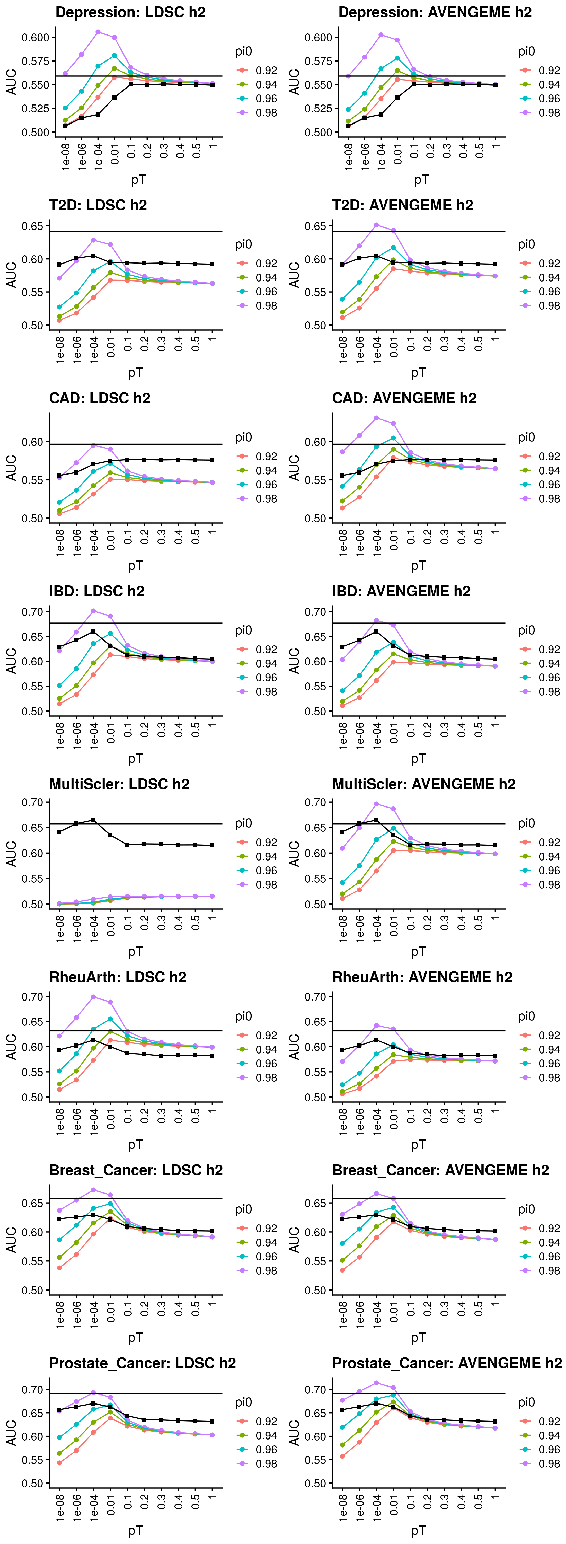
Phenotype	N	AVENGEME h2	LDSC h2	LDSC intercept	Prevalence	Sampling	Est. AUC (LDSC h2)	Est. AUC (AVENGEME h2)	Obs. AUC (pT1)	Obs. AUC (DBSLMM)
Depression	143265	0.097	0.100	0.997	0.150	0.318	0.567	0.565	0.549	0.559
T2D	152599	0.140	0.118	0.999	0.050	0.168	0.580	0.599	0.592	0.642
CAD	184305	0.078	0.055	0.887	0.030	0.330	0.559	0.590	0.576	0.597
IBD	34652	0.165	0.183	1.069	0.013	0.592	0.631	0.615	0.604	0.677
MultiScler	27148	0.133	0.020	1.062	0.002	0.360	0.515	0.623	0.615	0.657
RheuArth	58284	0.101	0.143	1.065	0.005	0.246	0.631	0.584	0.582	0.632
Breast_Cancer	228951	0.142	0.150	1.103	0.125	0.537	0.635	0.629	0.602	0.658
Prostate_Cancer	140254	0.218	0.188	1.081	0.125	0.564	0.652	0.673	0.632	0.691

Estimates of R2 using AVENGEME/LDSC

Etimation of PRS R2 using LDSC and AVENGEME approach

Phenotype	N	AVENGEME h2	LDSC h2	LDSC intercept	Est. R2 (LDSC h2)	Est. R2 (AVENGEME h2)	Obs. R2 (pT1)	Obs. R2 (DBSLMM)
Intelligence	95427	0.085	0.105	1.022	0.016	0.009	0.006	0.008
BMI	252064	0.178	0.312	1.328	0.236	0.108	0.058	0.081
Height	233681	0.183	0.130	0.672	0.063	0.110	0.063	0.110

---

2.1.2 GWIZ

We will calculate the AUC using GWIZ using the leave one out meta-analysis summary statistics, and then average the AUC results. This will hopefully tell us how much variance GWAS expects the LOO sumstats to explain in the left out subset.

---

2.1.2.1 Format GWAS summary statistics

Show code

library(data.table)

source('/users/k1806347/brc_scratch/Software/MyGit/GenoPred/config_used/Pipeline_prep.config')

pheno=c('Depression','T2D','CAD','IBD','MultiScler','RheuArth','Breast_Cancer','Prostate_Cancer')
gwas=c('DEPR07','DIAB05','COAD01','INFB01','SCLE03','RHEU02','BRCA01','PRCA01')
samp_prev=c(0.318,0.168,0.33,0.592,0.36,0.246,0.537,0.564)

dir.create('/scratch/users/k1806347/Analyses/AbsoluteRisk/Estimated_AUC_R2/GWIZ')

for(i in 1:length(pheno)){
  # Read in GWAS sumstats
  sumstats<-fread(paste0(gwas_rep_qcd,'/',gwas[i],'.cleaned.gz'))
  sumstats$phenotype<-'n/a'
  sumstats$dataset<-'n/a'
  sumstats$model<-'additive'
  
  if(sum(names(sumstats) == 'Ncas') == 0){
    sumstats$Ncas<-round(sumstats$N*samp_prev[i])
    sumstats$Ncon<-round(sumstats$N*(1-samp_prev[i]))
  }
  
  sumstats$control_size<-sumstats$Ncon
  sumstats$case_size<-sumstats$Ncas

  if(sum(names(sumstats) == 'REF.FREQ') > 0){
    sumstats$FREQ<-sumstats$REF.FREQ
    sumstats$REF.FREQ<-NULL
  }

  if(sum(names(sumstats) == 'OR') == 0){
    sumstats$OR<-exp(sumstats$BETA)
  }
  
  # OR and MAFs to all be corresponding to the risk allele
  sumstats$FREQ[sumstats$OR < 1]<-1-sumstats$FREQ[sumstats$OR < 1]
  names(sumstats)[names(sumstats) == 'FREQ']<-'risk_allele_freq'
  sumstats$BETA<-log(sumstats$OR)
  sumstats$OR[sumstats$OR < 1]<-exp(-sumstats$BETA[sumstats$OR < 1])
  
  # Extract LD independent variants
  ld_indep<-NULL
  for(chr in 1:22){
    ld_indep<-rbind(ld_indep, fread(paste0('/users/k1806347/brc_scratch/Data/1KG/Phase3/Score_files_for_polygenic/pt_clump/',gwas[i],'/1KGPhase3.w_hm3.',gwas[i],'.chr',chr,'.range_values')))
  }
  
  # Filter genome-wide variants 
  ld_indep_sig<-ld_indep[ld_indep$V2 < 1e-8]
  sumstats<-sumstats[(sumstats$SNP %in% ld_indep_sig$V1),]
  sumstats<-sumstats[,c('phenotype','dataset','SNP','control_size','case_size','risk_allele_freq','OR','model'),with=F]
  names(sumstats)[names(sumstats) == 'SNP']<-'accession'
  
  sumstats$model<-rep(c('recessive','dominant'),dim(sumstats)[1])[1:dim(sumstats)[1]]
  
  fwrite(sumstats, paste0('/scratch/users/k1806347/Analyses/AbsoluteRisk/Estimated_AUC_R2/GWIZ/',gwas[i],'.GWIZ.csv'), sep=',', na='NA', quote=F)
}

---

2.1.2.2 Run GWIZ

GWIZ is an R script. It needs to modification: - It doesn’t allow input files, software and output to be in different directories - It uses the png function which does’t work on Rosalind - It prints the contents of the GWAS sumstats repeatedly and GWIZ is an Rscript that must be modified to allow for different input and output files. I have edited the script slightly so all files don’t have be stored in the same directory, and can be easily run in parallel.

Show code

# Run GWIZ for each phenotype and subset
for gwas in $(echo DEPR07 DIAB05 COAD01 INFB01 SCLE03 RHEU02 BRCA01 PRCA01); do
    sbatch -p brc,shared --mem 10G /users/k1806347/brc_scratch/Software/Rscript.sh /users/k1806347/brc_scratch/Software/MyGit/GenoPred/Scripts/gwizer/gwizer.R \
      --sumstats /scratch/users/k1806347/Analyses/AbsoluteRisk/Estimated_AUC_R2/GWIZ/${gwas}.GWIZ.csv \
      --gwiz /mnt/lustre/users/k1806347/Software/GWIZ-Rscript-master \
      --output /scratch/users/k1806347/Analyses/AbsoluteRisk/Estimated_AUC_R2/GWIZ/${gwas}/res_${gwas}
done

---

2.1.2.3 Compare observed and estimate AUC

Show code

pheno=c('Depression','T2D','CAD','IBD','MultiScler','RheuArth','Breast_Cancer','Prostate_Cancer')
gwas=c('DEPR07','DIAB05','COAD01','INFB01','SCLE03','RHEU02','BRCA01','PRCA01')

AUC_comp<-NULL
for(i in 1:length(pheno)){
  GWIZ_AUC_i<-NULL
    GWIZ_AUC_i<-read.table(paste0('/scratch/users/k1806347/Analyses/AbsoluteRisk/Estimated_AUC_R2/GWIZ/',gwas[i],'/res_',gwas[i],'.log'), sep='&', header=F)$V1
    GWIZ_AUC_i_auc<-as.numeric(gsub('AUC = ','',GWIZ_AUC_i[grepl('AUC = ', GWIZ_AUC_i)]))
    
  pheno_res_pTclump<-fread(paste0('/scratch/users/k1806347/Analyses/AbsoluteRisk/Measured_AUC_R2/',pheno[i],'/UKBB.w_hm3.',gwas[i],'.EUR-PRSs.AllMethodComp.assoc.txt'))

  Obs_AUC<-pheno_res_pTclump$AUC[grepl('pT.clump', pheno_res_pTclump$Predictor) & grepl('1e.06', pheno_res_pTclump$Predictor)]
  
  AUC_comp<-rbind(AUC_comp, data.frame(Phenotype=pheno[i],
                                       Obs_AUC=Obs_AUC,
                                       GWIZ_AUC=GWIZ_AUC_i_auc))
}

write.csv(AUC_comp, '/scratch/users/k1806347/Analyses/AbsoluteRisk/Estimated_AUC_R2/GWIZ_AUC.csv', row.names=F, quote=F)

# GWIZ is not performing well, except for T2D, CAD, IBD, and Depression. Again, I think this might be due to improper preparation of GWAS summary statistics. GWIZ is also running quite slow, and would need to be run GW to get accurate estimates for polygenic outcomes. I don't think this is a viable option. This method is also not suitable for continous outcomes.

Show results

Estimation of PRS AUC using GWIZ

Phenotype	Obs_AUC	GWIZ_AUC
Depression	0.5149628	0.5046247
T2D	0.6011381	0.5715527
CAD	0.5598304	0.5610959
IBD	0.6424438	0.6745935
MultiScler	0.6577221	0.5523625
RheuArth	0.6024688	0.7521208
Breast_Cancer	0.6258635	0.7565655
Prostate_Cancer	0.6631618	0.8004651

---

2.1.3 Lassosum

Lassosum has a pseudovalidate option which estimates the correlation between predicted and observed values across shrinkage parameters. Although, its ability to estimate the best shrinakge parameter, the estimated correlation for the top shrinkage parameter appears similar to the observed correlation. We can convert the correlation into an R2 for continuous outcomes, and possible into an AUC, but converting to observed R2 into a liability R2, and then into an AUC. This would also be more suitable to predicting R2/AUC for the more modern shrinkage PRS methods, since lassosum is one.

---

2.1.3.1 Pseudovalidate

Show code

. /users/k1806347/brc_scratch/Software/MyGit/GenoPred/config_used/Pipeline_prep.config

##########
# Run excluding MHC
##########

# Create directory
mkdir /scratch/users/k1806347/Analyses/AbsoluteRisk/Estimated_AUC_R2/lassosum

# Create file listing GWAS that haven't been processed.
> /scratch/users/k1806347/Analyses/AbsoluteRisk/Estimated_AUC_R2/lassosum/todo_noMHC.txt
for gwas in $(echo DEPR07 COLL01 BODY04 HEIG03 DIAB05 COAD01 INFB01 SCLE03 RHEU02 BRCA01 PRCA01);do
if [ ! -f /scratch/users/k1806347/Analyses/AbsoluteRisk/Estimated_AUC_R2/lassosum/${gwas}_noMHC/lassosum_pseudo_${gwas}.pseudovalidate.png ]; then
echo $gwas >> /scratch/users/k1806347/Analyses/AbsoluteRisk/Estimated_AUC_R2/lassosum/todo_noMHC.txt
fi
done

# Create shell script to run using sbatch
cat > /scratch/users/k1806347/Analyses/AbsoluteRisk/Estimated_AUC_R2/lassosum/sbatch_noMHC.sh << 'EOF'
#!/bin/sh

#SBATCH -p shared,brc
#SBATCH --mem=10G
#SBATCH -n 1
#SBATCH -J lassosum

. /users/k1806347/brc_scratch/Software/MyGit/GenoPred/config_used/Pipeline_prep.config

gwas=$(sed "${SLURM_ARRAY_TASK_ID}q;d" /scratch/users/k1806347/Analyses/AbsoluteRisk/Estimated_AUC_R2/lassosum/todo_noMHC.txt)
echo ${gwas}

/users/k1806347/brc_scratch/Software/Rscript.sh /users/k1806347/brc_scratch/Software/MyGit/GenoPred/Scripts/lassosum_pseudovalidate/lassosum_pseudovalidate.R \
    --ref_plink_gw ${Geno_1KG_dir}/1KGPhase3.w_hm3.GW \
    --ref_keep ${Geno_1KG_dir}/keep_files/EUR_samples.keep \
  --sumstats ${gwas_rep_qcd}/${gwas}.cleaned.gz \
  --prune_mhc T \
    --output /scratch/users/k1806347/Analyses/AbsoluteRisk/Estimated_AUC_R2/lassosum/${gwas}_noMHC/lassosum_pseudo_${gwas} \
    --plink /users/k1806347/brc_scratch/Software/plink1.9.sh \
    --n_cores 1
EOF

sbatch --array 1-$(wc -l /scratch/users/k1806347/Analyses/AbsoluteRisk/Estimated_AUC_R2/lassosum/todo_noMHC.txt | cut -d' ' -f1)%5 /scratch/users/k1806347/Analyses/AbsoluteRisk/Estimated_AUC_R2/lassosum/sbatch_noMHC.sh

---

2.1.3.2 Compare observed and estimate AUC

Show code

library(data.table)

#####
# Binary outcomes
#####
pheno=c('Depression','T2D','CAD','IBD','MultiScler','RheuArth','Breast_Cancer','Prostate_Cancer')
gwas=c('DEPR07','DIAB05','COAD01','INFB01','SCLE03','RHEU02','BRCA01','PRCA01')
samp_prev=c(0.318,0.168,0.33,0.592,0.36,0.246,0.537,0.564,0.318)

AUC_comp<-NULL
for(i in 1:length(pheno)){
  lasso_AUC_i<-NULL
  lasso_AUC_i<-read.table(paste0('/scratch/users/k1806347/Analyses/AbsoluteRisk/Estimated_AUC_R2/lassosum/',gwas[i],'_noMHC/lassosum_pseudo_',gwas[i],'.log'), sep='&', header=F)$V1
  lasso_AUC_i_r<-as.numeric(gsub('value = ','',lasso_AUC_i[grepl('value = ', lasso_AUC_i)]))
  
  n_case<-samp_prev[i]
  n_con<-1-samp_prev[i]
  
  a<-(n_case+n_con)^2/(n_case*n_con)
  
  lasso_AUC_i_d<-sqrt(a)*lasso_AUC_i_r/sqrt(1-lasso_AUC_i_r^2)
  lasso_AUC_i_auc <- pnorm(lasso_AUC_i_d/sqrt(2), 0, 1)
  
  pheno_res<-fread(paste0('/scratch/users/k1806347/Analyses/AbsoluteRisk/Measured_AUC_R2/',pheno[i],'/UKBB.w_hm3.',gwas[i],'.EUR-PRSs.AllMethodComp.assoc.txt'))

  Obs_pT_clump_AUC<-pheno_res$AUC[grepl('_1$', pheno_res$Predictor)]
  Obs_DBSLMM_AUC<-pheno_res$AUC[grepl('_DBSLMM', pheno_res$Predictor)]

  AUC_comp<-rbind(AUC_comp, data.frame(Phenotype=pheno[i],
                                       Obs_pTclump_pt1_AUC=Obs_pT_clump_AUC,
                                       Obs_DBSLMM_AUC=Obs_DBSLMM_AUC,
                                       Est_lasso_AUC=lasso_AUC_i_auc))
}

AUC_comp$Est_Obs_diff_DBSLMM<-AUC_comp$Est_lasso_AUC-AUC_comp$Obs_DBSLMM_AUC

write.csv(AUC_comp, '/scratch/users/k1806347/Analyses/AbsoluteRisk/Estimated_AUC_R2/lassosum/lassosum_AUC.csv', row.names=F, quote=F)

#####
# Continuous outcomes
#####
pheno=c('Intelligence','BMI','Height')
gwas=c('COLL01','BODY04','HEIG03')

R2_comp<-NULL
for(i in 1:length(pheno)){
    lasso_R2_i<-NULL
    lasso_R2_i<-read.table(paste0('/scratch/users/k1806347/Analyses/AbsoluteRisk/Estimated_AUC_R2/lassosum/',gwas[i],'_noMHC/lassosum_pseudo_',gwas[i],'.log'), sep='&', header=F)$V1
    lasso_R2_i_r<-as.numeric(gsub('value = ','',lasso_R2_i[grepl('value = ', lasso_R2_i)]))
    
    lasso_R2_i_r2<-lasso_R2_i_r^2

    pheno_res<-fread(paste0('/scratch/users/k1806347/Analyses/AbsoluteRisk/Measured_AUC_R2/',pheno[i],'/UKBB.w_hm3.',gwas[i],'.EUR-PRSs.AllMethodComp.assoc.txt'))
  
    Obs_pT_clump_R2<-pheno_res$Obs_R2[grepl('_1$', pheno_res$Predictor)]
    Obs_DBSLMM_R2<-pheno_res$Obs_R2[grepl('_DBSLMM', pheno_res$Predictor)]
    
    R2_comp<-rbind(R2_comp, data.frame(Phenotype=pheno[i],
                                         Obs_pTclump_pT1_R2=Obs_pT_clump_R2,
                                         Obs_DBSLMM_R2=Obs_DBSLMM_R2,
                                         lasso_R2=lasso_R2_i_r2))
}

R2_comp$Est_Obs_diff_DBSLMM<-R2_comp$lasso_R2-R2_comp$Obs_DBSLMM_R2

write.csv(R2_comp, '/scratch/users/k1806347/Analyses/AbsoluteRisk/Estimated_AUC_R2/lassosum/lassosum_R2.csv', row.names=F, quote=F)

# This is looking really promising. Lassosum has some trouble with IBD, MultiScler and RheuArth, but otherwise is very accurate. These outcomes are all rarer and autoimmune disorders. I have run without mhc region but results still poor for these outcomes. Discordant findings may be due to phenotype heterogeneity between GWAS and UKB.

Show results

Estimation of PRS AUC using lassosum

Phenotype	Observed AUC	Estimated AUC	Difference
Depression	0.559	0.555	-0.004
T2D	0.642	0.651	0.010
CAD	0.597	0.624	0.027
IBD	0.677	0.792	0.115
MultiScler	0.657	0.785	0.128
RheuArth	0.632	0.500	-0.132
Breast_Cancer	0.658	0.698	0.040
Prostate_Cancer	0.691	0.721	0.030

Estimation of PRS R2 using lassosum

Phenotype	Observed R2	Estimated R2	Difference
Intelligence	0.008	0.023	0.015
BMI	0.081	0.074	-0.007
Height	0.110	0.156	0.046

---

Based on these results, none of these approaches are brilliant. The AVENGEME/LDSC method is limited by the accuracy of the LDSC heritability estimate, and the ‘medium’ polygencity assumed by using a pi0 of 0.94. The lassosum approach does fairly well, but is not good for the autoimmune disorders. I think we should use the lassosum estimate unless it is R2=0 or AUC=0.5.

---

2.1.4 Compare absolute estimates/values when using AVENGEME AUC/R2

---

2.1.4.1 Binary

Show code

library(data.table)

source('/users/k1806347/brc_scratch/Software/MyGit/GenoPred/config_used/Target_scoring.config')

pheno=c('Depression','T2D','CAD','IBD','MultiScler','RheuArth','Breast_Cancer','Prostate_Cancer')
gwas=c('DEPR07','DIAB05','COAD01','INFB01','SCLE03','RHEU02','BRCA01','PRCA01')

n_quant<-20

files<-data.frame(pheno,gwas)

# Create function
ccprobs.f <- function(PRS_auc=0.641, prev=0.7463, n_quantile=20){
  
    # Convert AUC into cohen's d
    d <- sqrt(2)*qnorm(PRS_auc)
    
    # Set mean difference between cases and control polygenic scores
    mu_case <- d
    mu_control <- 0
    
    # Estimate mean and variance of polygenic scores across case and control
    varPRS <- prev*(1+(d^2) - (d*prev)^2) + (1-prev)*(1 - (d*prev)^2)
    E_PRS <- d*prev
    
    # Estimate polygenic score quantiles
    by_quant<-1/n_quantile
    p_quant <- seq(by_quant, 1-by_quant, by=by_quant)
    quant_vals_PRS <- rep(0, length(p_quant))
    quant_f_solve <- function(x, prev, d, pq){prev*pnorm(x-d) + (1-prev)*pnorm(x) - pq}
    for(i in 1:length(p_quant)){
        quant_vals_PRS[i] <- unlist(uniroot(quant_f_solve, prev=prev, d=d, pq= p_quant[i], interval=c(-2.5, 2.5), extendInt = "yes", tol=6e-12)$root)
    }
    
    # Create a table for output
    ul_qv_PRS <- matrix(0, ncol=2, nrow=n_quantile)
    ul_qv_PRS[1,1] <- -Inf
    ul_qv_PRS[2:n_quantile,1] <- quant_vals_PRS
    ul_qv_PRS[1:(n_quantile-1),2] <- quant_vals_PRS
    ul_qv_PRS[n_quantile,2] <- Inf
    
    ul_qv_PRS<-cbind(ul_qv_PRS, (ul_qv_PRS[,1:2]-E_PRS)/sqrt(varPRS))
    
    # Estimate case control proportion for each quantile
    prob_quantile_case <- pnorm(ul_qv_PRS[,2], mean = mu_case) - pnorm(ul_qv_PRS[,1], mean = mu_case)
    prob_quantile_control <- pnorm(ul_qv_PRS[,2], mean = mu_control) - pnorm(ul_qv_PRS[,1], mean = mu_control)
    p_case_quantile <- (prob_quantile_case*prev)/by_quant
    p_cont_quantile <- (prob_quantile_control*(1-prev))/by_quant
    
    # Estimate OR comparing each quantile to bottom quantile
    OR <- p_case_quantile/p_cont_quantile
    OR <- OR/OR[1]
    
    # Return output
    out <- cbind(ul_qv_PRS[,3:4],p_cont_quantile, p_case_quantile, OR)
    row.names(out) <- 1:n_quantile
    colnames(out) <- c("q_min", "q_max","p_control", "p_case", "OR")
    
    data.frame(out)
}

# Read in AVENGEME AUC
AVENGEME_AUC<-read.csv('/scratch/users/k1806347/Analyses/AbsoluteRisk/Estimated_AUC_R2/AVENGEME_AUC.csv')

# Run analysis for each phenotype
res_all<-NULL
cor_res<-NULL
plots_all<-list()

for(i in 1:dim(files)[1]){
  # Read in pheno and prs data, and merge
  pheno_i<-fread(paste0(UKBB_output,'/Phenotype/PRS_comp_subset/UKBB.',files$pheno[i],'.txt'))
  names(pheno_i)[3]<-'pheno'
  prs_i<-fread(paste0(UKBB_output,'/PRS_for_interpretation/1KG_ref/DBSLMM/',files$gwas[i],'/UKBB.subset.w_hm3.',files$gwas[i],'.DBSLMM_profiles'))
  prs_i<-prs_i[,c('FID','IID',paste0(files$gwas[i], '_DBSLMM')), with=F]
  names(prs_i)[3]<-'prs'

  pheno_prs<-merge(pheno_i, prs_i, by=c('FID','IID'))
  
  # Read in AUC for PRS
  assoc<-fread(paste0('/scratch/users/k1806347/Analyses/AbsoluteRisk/Measured_AUC_R2/',files$pheno[i],'/UKBB.w_hm3.',files$gwas[i],'.EUR-PRSs.AllMethodComp.assoc.txt'))
  prs_auc<-assoc[grepl('DBSLMM', assoc$Predictor),]$AUC
  
  # Assign individuals to observed PRS quantiles
  obs_quant<-quantile(pheno_prs$prs, prob = seq(0, 1, length = n_quant+1))
  pheno_prs$obs_quant<-as.numeric(cut( pheno_prs$prs, obs_quant, include.lowest = T))

  # Calculate proportion of each quantile that are cases
  obs_cc<-NULL
  for(k in 1:n_quant){
    obs_cc<-rbind(obs_cc, data.frame(Phenotype=files$pheno[i],
                                     Type='Observed',
                                     Quantile=k,
                                     q_min=obs_quant[k],
                                     q_max=obs_quant[k+1],
                                     p_control=1-mean(pheno_prs$pheno[pheno_prs$obs_quant == k]),
                                     p_case=mean(pheno_prs$pheno[pheno_prs$obs_quant == k])))
  }
  
  # Assign individuals to estimated PRS quantiles
  est_cc<-ccprobs.f(PRS_auc = prs_auc, prev=mean(pheno_prs$pheno), n_quantile = n_quant)
  est_cc$OR<-NULL
  est_cc<-data.frame(Phenotype=files$pheno[i],Type='Estimated',Quantile=1:n_quant, est_cc)
  est_quant<-sort(unique(c(est_cc$q_min, est_cc$q_max)))
  pheno_prs$est_quant<-as.numeric(cut( pheno_prs$prs, est_quant, include.lowest = T))
  
  tmp<-cor.test(obs_cc$p_case, est_cc$p_case)
  tmp2<-abs(est_cc$p_case-obs_cc$p_case)/obs_cc$p_case

  # Assign individuals to estimated PRS quantiles
  AVENGEME_est_cc<-ccprobs.f(PRS_auc = AVENGEME_AUC$pred_AUC_LDSC[AVENGEME_AUC$Phenotype == files$pheno[i]], prev=mean(pheno_prs$pheno), n_quantile = n_quant)
  AVENGEME_est_cc$OR<-NULL
  AVENGEME_est_cc<-data.frame(Phenotype=files$pheno[i],Type="Estimated\n(AVENGEME)",Quantile=1:n_quant, AVENGEME_est_cc)
  AVENGEME_est_quant<-sort(unique(c(AVENGEME_est_cc$q_min, AVENGEME_est_cc$q_max)))
  pheno_prs$AVENGEME_est_quant<-as.numeric(cut( pheno_prs$prs, AVENGEME_est_quant, include.lowest = T))

  tmp3<-cor.test(obs_cc$p_case, AVENGEME_est_cc$p_case)
  tmp4<-abs(AVENGEME_est_cc$p_case-obs_cc$p_case)/obs_cc$p_case
  
  # Estimate correlation between observed and expected
  cor_res<-rbind(cor_res,data.frame(Phenotype=files$pheno[i],
                                    Cor=tmp$estimate,
                                    Low95CI=tmp$conf.int[1],
                                    High95CI=tmp$conf.int[2],
                                    Mean_perc_diff=mean(tmp2),
                                    Cor_AVENGEME=tmp3$estimate,
                                    Low95CI_AVENGEME=tmp3$conf.int[1],
                                    High95CI_AVENGEME=tmp3$conf.int[2],
                                    Mean_perc_diff_AVENGEME=mean(tmp4),
                                    N=length(pheno_prs$pheno),
                                    Ncas=sum(pheno_prs$pheno == 1),
                                    Ncon=sum(pheno_prs$pheno == 0)))

  quant_comp<-do.call(rbind,list(obs_cc, est_cc, AVENGEME_est_cc))
  
  res_all<-rbind(res_all, quant_comp)
  
  library(ggplot2)
  library(cowplot)
  
  plots_all[[i]]<-ggplot(quant_comp, aes(x=Quantile, y=p_case, colour=Type)) +
                    geom_point(alpha=0.8) +
                    geom_line(alpha=0.8) +
                    labs(x='PRS quantile', y=paste0('Proportion with ',files$pheno[i]), title=files$pheno[i], colour='Method') +
                    theme_cowplot(12)
}

png(paste0('/scratch/users/k1806347/Analyses/AbsoluteRisk/Measured_AUC_R2/PropCC_Comp_AVENGEME.png'), units='px', res=300, width=2000, height=3000)
  plot_grid(plotlist=plots_all, ncol = 2)
dev.off()

write.csv(cor_res, '/scratch/users/k1806347/Analyses/AbsoluteRisk/Measured_AUC_R2/PropCC_Comp_AVENGEME.csv', row.names=F, quote=F)

ex_est<-res_all[res_all$Phenotype == 'MultiScler' & res_all$Type == "Estimated\n(AVENGEME)" & res_all$Quantile == 20,]$p_case
ex_obs<-res_all[res_all$Phenotype == 'MultiScler' & res_all$Type == 'Observed' & res_all$Quantile == 20,]$p_case
ex_est/ex_obs

ex_est<-res_all[res_all$Phenotype == 'IBD' & res_all$Type == "Estimated\n(AVENGEME)" & res_all$Quantile == 20,]$p_case
ex_obs<-res_all[res_all$Phenotype == 'IBD' & res_all$Type == 'Observed' & res_all$Quantile == 20,]$p_case
ex_est/ex_obs

ex_est<-res_all[res_all$Phenotype == 'T2D' & res_all$Type == "Estimated\n(AVENGEME)" & res_all$Quantile == 20,]$p_case
ex_obs<-res_all[res_all$Phenotype == 'T2D' & res_all$Type == 'Observed' & res_all$Quantile == 20,]$p_case
ex_est/ex_obs

Show results

Correlation between observed and estimated proportion of cases within polygenic score quantiles

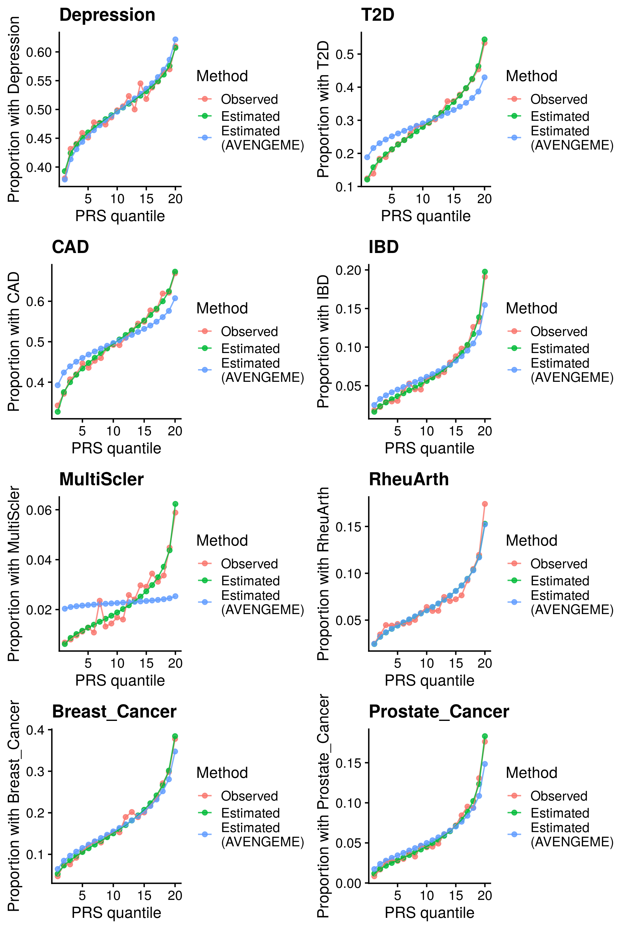
Phenotype	Cor	Low95CI	High95CI	Mean_perc_diff	Cor_AVENGEME	Low95CI_AVENGEME	High95CI_AVENGEME	Mean_perc_diff_AVENGEME	N	Ncas	Ncon
Depression	0.9845782	0.9605776	0.9940117	0.0150485	0.9844983	0.9603757	0.9939806	0.0193074	49999	24999	25000
T2D	0.9968126	0.9917731	0.9987670	0.0236348	0.9968601	0.9918954	0.9987854	0.1530956	49999	14888	35111
CAD	0.9943181	0.9853636	0.9978003	0.0153319	0.9938163	0.9840773	0.9976057	0.0578957	49999	25000	24999
IBD	0.9941885	0.9850314	0.9977501	0.0683969	0.9928430	0.9815852	0.9972280	0.1825526	49999	3461	46538
MultiScler	0.9691668	0.9221227	0.9879704	0.1262171	0.9375296	0.8459902	0.9753859	0.6005559	49999	1137	48862
RheuArth	0.9813043	0.9523309	0.9927332	0.0684472	0.9810557	0.9517064	0.9926360	0.0678404	49999	3408	46591
Breast_Cancer	0.9949234	0.9869165	0.9980350	0.0456799	0.9955383	0.9884957	0.9982734	0.0838627	49999	8512	41487
Prostate_Cancer	0.9939174	0.9843364	0.9976449	0.0870004	0.9930048	0.9819994	0.9972908	0.1788078	50000	2927	47073

Median Cor. = 0.9929239; Mean Cor. = 0.9843933; Min. Cor. = 0.9375296; Max. Cor. = 0.9968601

Excluding RheuArth: Median Cor. = 0.9930048; Mean Cor. = 0.98487; Min. Cor. = 0.9375296; Max. Cor. = 0.9968601

---

2.1.4.2 Continuous

Show code

library(data.table)
library(e1071)

source('/users/k1806347/brc_scratch/Software/MyGit/GenoPred/config_used/Target_scoring.config')

gwas<-c('COLL01','HEIG03','BODY04')
pheno<-c('Intelligence','Height','BMI')

n_quant<-20

files<-data.frame(pheno,gwas)

# Create function
mean_sd_quant.f <- function(PRS_R2=0.641, Outcome_mean=1, Outcome_sd=1, n_quantile=20){
  ### PRS quantiles with a continuous phenotype (Y)
  library(tmvtnorm)
  ###
  E_PRS = 0
  SD_PRS = sqrt(1)
  E_phenotype = Outcome_mean
  SD_phenotype = Outcome_sd 

  by_quant<-1/(n_quantile)
  PRS_quantile_bounds <- qnorm(p=seq(0, 1, by=by_quant), mean= E_PRS, sd= SD_PRS)
  lower_PRS_vec <- PRS_quantile_bounds[1:n_quantile]
  upper_PRS_vec <- PRS_quantile_bounds[2:(n_quantile+1)]
  
  mean_vec <- c(E_phenotype, E_PRS)
  sigma_mat <- matrix(sqrt(PRS_R2)*SD_phenotype*SD_PRS, nrow=2, ncol=2)
  sigma_mat[1,1] <- SD_phenotype^2
  sigma_mat[2,2] <- SD_PRS^2
  
  ### mean of phenotype within the truncated PRS distribution
  out_mean_Y <- rep(0, 20)
  ### SD of phenotype within the truncated PRS distribution
  out_SD_Y <- rep(0, 20)
  ### cov of Y and PRS given truncation on PRS
  out_cov_Y_PRS <- rep(0, 20)
  ### SD of PRS given truncation on PRS
  out_SD_PRS <- rep(0, 20)
  ### mean PRS given truncation on PRS
  out_mean_PRS <- rep(0, 20)
  
  for(i in 1:n_quantile){
    distribution_i <- mtmvnorm(mean = mean_vec,
        sigma = sigma_mat,
        lower = c(-Inf, lower_PRS_vec[i]),
        upper = c(Inf, upper_PRS_vec[i]),
        doComputeVariance=TRUE,
        pmvnorm.algorithm=GenzBretz())
        out_mean_Y[i] <- distribution_i$tmean[1]
        out_mean_PRS[i] <- distribution_i$tmean[2]
        out_SD_Y[i] <- sqrt(distribution_i$tvar[1,1])
        out_SD_PRS[i] <- sqrt(distribution_i$tvar[2,2])
        out_cov_Y_PRS[i] <- distribution_i$tvar[1,2]
  }
  
  out<-data.frame(q=1:n_quantile,
             q_min=lower_PRS_vec,
             q_max=upper_PRS_vec,
             x_mean=out_mean_Y,
             x_sd=out_SD_Y)
  
  return(out)

  out_mean_Y
  out_SD_Y
  
  out_mean_PRS
  out_SD_PRS
  out_cov_Y_PRS
}

# Read in AVENGEME R2
AVENGEME_R2<-read.csv('/scratch/users/k1806347/Analyses/AbsoluteRisk/Estimated_AUC_R2/AVENGEME_R2.csv')

# Run analysis for each phenotype
res_all<-NULL
plots_all<-list()
cor_res<-NULL

for(i in 1:dim(files)[1]){
  # Read in pheno and prs data, and merge
  pheno_i<-fread(paste0(UKBB_output,'/Phenotype/PRS_comp_subset/UKBB.',files$pheno[i],'.txt'))
  names(pheno_i)[3]<-'pheno'
  prs_i<-fread(paste0(UKBB_output,'/PRS_for_interpretation/1KG_ref/DBSLMM/',files$gwas[i],'/UKBB.subset.w_hm3.',files$gwas[i],'.DBSLMM_profiles'))
  prs_i<-prs_i[,c('FID','IID',paste0(files$gwas[i], '_DBSLMM')), with=F]
  names(prs_i)[3]<-'prs'

  pheno_prs<-merge(pheno_i, prs_i, by=c('FID','IID'))
  
  # Read in AUC for PRS
  assoc<-fread(paste0('/scratch/users/k1806347/Analyses/AbsoluteRisk/Measured_AUC_R2/',files$pheno[i],'/UKBB.w_hm3.',files$gwas[i],'.EUR-PRSs.AllMethodComp.assoc.txt'))
  prs_r2<-assoc[grepl('DBSLMM', assoc$Predictor),]$Obs_R2
  
  # Assign individuals to observed PRS quantiles
  obs_quant<-quantile(pheno_prs$prs, prob = seq(0, 1, length = n_quant+1))
  pheno_prs$obs_quant<-as.numeric(cut( pheno_prs$prs, obs_quant, include.lowest = T))

  # Calculate mean and SD of each quantile that are cases
  obs_dist<-NULL
  for(k in 1:n_quant){
    obs_dist<-rbind(obs_dist, data.frame(Phenotype=files$pheno[i],
                                     Type='Observed',
                                     Quantile=k,
                                     q_min=obs_quant[k],
                                     q_max=obs_quant[k+1],
                                     x_mean=mean(pheno_prs$pheno[pheno_prs$obs_quant == k]),
                                     x_sd=sd(pheno_prs$pheno[pheno_prs$obs_quant == k])))
  }
  
  # Assign individuals to estimated PRS quantiles
  est_dist<-mean_sd_quant.f(PRS_R2 = prs_r2, Outcome_mean=mean(pheno_prs$pheno), Outcome_sd=sd(pheno_prs$pheno), n_quantile = n_quant)
  est_dist$q<-NULL
  est_dist<-data.frame(Phenotype=files$pheno[i],Type='Estimated',Quantile=1:n_quant, est_dist)
  est_quant<-sort(unique(c(est_dist$q_min, est_dist$q_max)))
  pheno_prs$est_quant<-as.numeric(cut( pheno_prs$prs, est_quant, include.lowest = T))

  # Assign individuals to AVENGEME estimated PRS quantiles
  AVENGEME_est_dist<-mean_sd_quant.f(PRS_R2 = AVENGEME_R2$pred_R2_LDSC[AVENGEME_R2$Phenotype == files$pheno[i]], Outcome_mean=mean(pheno_prs$pheno), Outcome_sd=sd(pheno_prs$pheno), n_quantile = n_quant)
  AVENGEME_est_dist$q<-NULL
  AVENGEME_est_dist<-data.frame(Phenotype=files$pheno[i],Type="Estimated\n(AVENGEME)",Quantile=1:n_quant, AVENGEME_est_dist)
  AVENGEME_est_quant<-sort(unique(c(AVENGEME_est_dist$q_min, AVENGEME_est_dist$q_max)))
  pheno_prs$AVENGEME_est_quant<-as.numeric(cut( pheno_prs$prs, AVENGEME_est_quant, include.lowest = T))
  
  quant_comp<-do.call(rbind, list(obs_dist, est_dist, AVENGEME_est_dist))
  
  tmp<-cor.test(obs_dist$x_mean, est_dist$x_mean)
  tmp2<-cor.test(obs_dist$x_mean, AVENGEME_est_dist$x_mean)
  
  cor_res<-rbind(cor_res,data.frame(Phenotype=files$pheno[i],
                                    Cor_mean=tmp$estimate,
                                    Cor_mean_Low95CI=tmp$conf.int[1],
                                    Cor_mean_High95CI=tmp$conf.int[2],
                                    Cor_mean_AVENGEME=tmp2$estimate,
                                    Cor_mean_Low95CI_AVENGEME=tmp2$conf.int[1],
                                    Cor_mean_High95CI_AVENGEME=tmp2$conf.int[2],
                                    PercDiff_sd_mean=mean(abs(est_dist$x_sd-obs_dist$x_sd)/obs_dist$x_sd),
                                    PercDiff_sd_mean_AVENGEME=mean(abs(AVENGEME_est_dist$x_sd-obs_dist$x_sd)/obs_dist$x_sd),
                                    N=length(pheno_prs$pheno),
                                    Skewness=skewness(pheno_prs$pheno)))

  res_all<-rbind(res_all, quant_comp)
  
  library(ggplot2)
  library(cowplot)
  
  plots_all[[i]]<-ggplot(quant_comp, aes(x=Quantile, y=x_mean, colour=Type)) +
    geom_point(stat="identity", position=position_dodge(.9), alpha=0.8, shape=18) +
    geom_errorbar(aes(ymin=x_mean-x_sd, ymax=x_mean+x_sd), width=.2, position=position_dodge(.9), alpha=0.8) +
    labs(x='PRS quantile', y=paste0(pheno[i], " mean (SD)"), title=files$pheno[i], colour='Method') +
    theme_cowplot(12)
  
}

png(paste0('/scratch/users/k1806347/Analyses/AbsoluteRisk/Measured_AUC_R2/Mean_SD_Comp_AVENGEME.png'), units='px', res=300, width=1500, height=1750)
  plot_grid(plotlist=plots_all, ncol = 1)
dev.off()

write.csv(cor_res, '/scratch/users/k1806347/Analyses/AbsoluteRisk/Measured_AUC_R2/Mean_SD_Comp_AVENGEME.csv', row.names=F, quote=F)

Show results

Correlation between observed and estimated mean and standar deviation of outcome within polygenic score quantiles

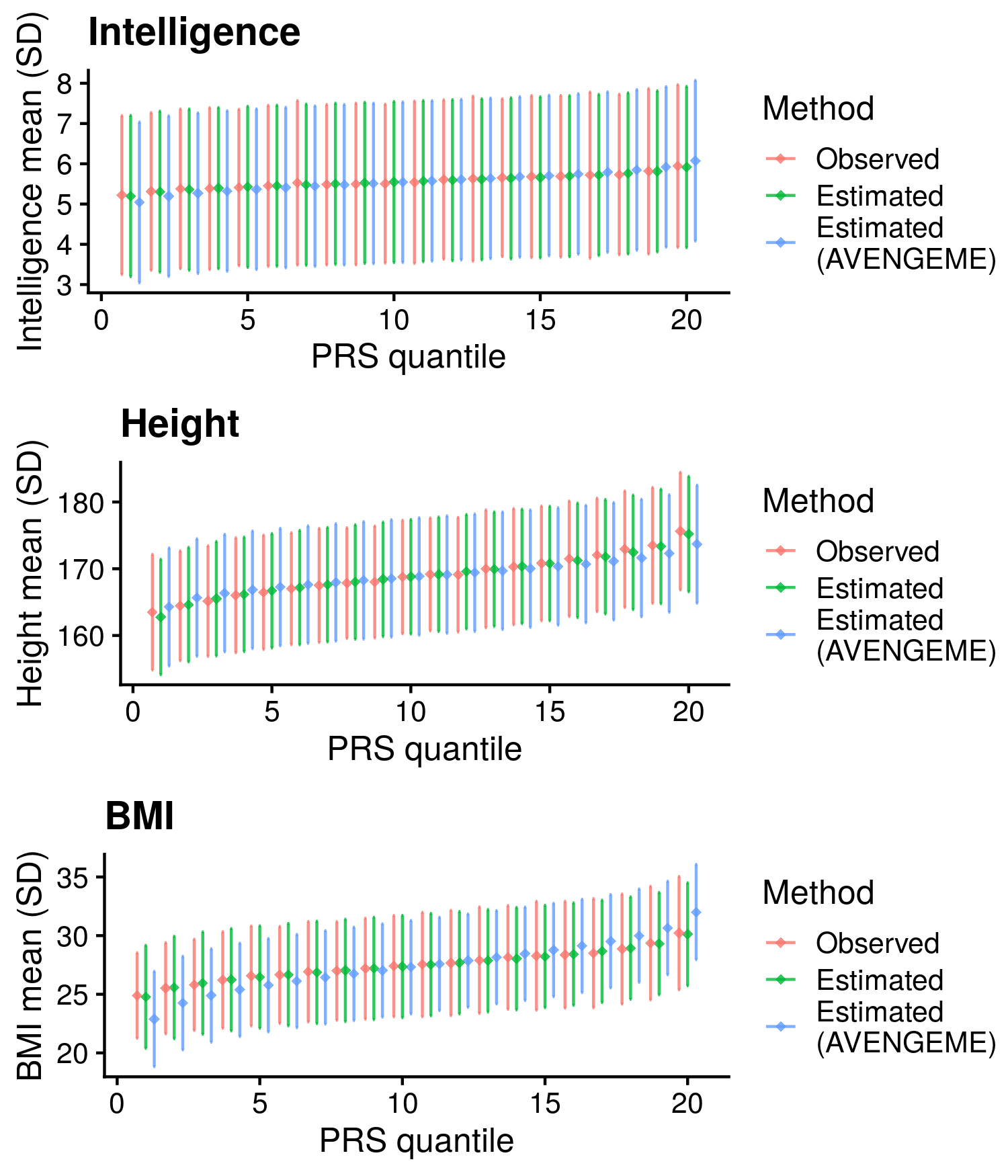
Phenotype	Cor_mean	Cor_mean_Low95CI	Cor_mean_High95CI	Cor_mean_AVENGEME	Cor_mean_Low95CI_AVENGEME	Cor_mean_High95CI_AVENGEME	PercDiff_sd_mean	PercDiff_sd_mean_AVENGEME	N	Skewness
Intelligence	0.9917264	0.9787310	0.9967944	0.9917264	0.9787310	0.9967944	0.0132982	0.0135699	50000	0.1440539
Height	0.9958381	0.9892663	0.9983895	0.9958381	0.9892663	0.9983895	0.0151424	0.0306504	49999	0.1168512
BMI	0.9981713	0.9952749	0.9992929	0.9981713	0.9952749	0.9992929	0.0596993	0.0959049	49999	0.5915969

Median Cor. of means = 0.9958381; Mean Cor. of means = 0.9952452; Min. Cor. of means = 0.9917264; Max. Cor. of means = 0.9981713

Median mean %diff of SD = 0.03065044; Mean mean %diff of SD = 0.04670842; Min. mean %diff of SD = 0.01356991; Max. mean %diff of SD = 0.09590491

---

2.1.5 Compare absolute estimates/values when using lassosum AUC/R2

---

2.1.5.1 Binary

Show code

library(data.table)

source('/users/k1806347/brc_scratch/Software/MyGit/GenoPred/config_used/Target_scoring.config')

pheno=c('Depression','T2D','CAD','IBD','MultiScler','RheuArth','Breast_Cancer','Prostate_Cancer')
gwas=c('DEPR07','DIAB05','COAD01','INFB01','SCLE03','RHEU02','BRCA01','PRCA01')

n_quant<-20

files<-data.frame(pheno,gwas)

# Create function
ccprobs.f <- function(PRS_auc=0.641, prev=0.7463, n_quantile=20){
  
    # Convert AUC into cohen's d
    d <- sqrt(2)*qnorm(PRS_auc)
    
    # Set mean difference between cases and control polygenic scores
    mu_case <- d
    mu_control <- 0
    
    # Estimate mean and variance of polygenic scores across case and control
    varPRS <- prev*(1+(d^2) - (d*prev)^2) + (1-prev)*(1 - (d*prev)^2)
    E_PRS <- d*prev
    
    # Estimate polygenic score quantiles
    by_quant<-1/n_quantile
    p_quant <- seq(by_quant, 1-by_quant, by=by_quant)
    quant_vals_PRS <- rep(0, length(p_quant))
    quant_f_solve <- function(x, prev, d, pq){prev*pnorm(x-d) + (1-prev)*pnorm(x) - pq}
    for(i in 1:length(p_quant)){
        quant_vals_PRS[i] <- unlist(uniroot(quant_f_solve, prev=prev, d=d, pq= p_quant[i], interval=c(-2.5, 2.5), extendInt = "yes", tol=6e-12)$root)
    }
    
    # Create a table for output
    ul_qv_PRS <- matrix(0, ncol=2, nrow=n_quantile)
    ul_qv_PRS[1,1] <- -Inf
    ul_qv_PRS[2:n_quantile,1] <- quant_vals_PRS
    ul_qv_PRS[1:(n_quantile-1),2] <- quant_vals_PRS
    ul_qv_PRS[n_quantile,2] <- Inf
    
    ul_qv_PRS<-cbind(ul_qv_PRS, (ul_qv_PRS[,1:2]-E_PRS)/sqrt(varPRS))
    
    # Estimate case control proportion for each quantile
    prob_quantile_case <- pnorm(ul_qv_PRS[,2], mean = mu_case) - pnorm(ul_qv_PRS[,1], mean = mu_case)
    prob_quantile_control <- pnorm(ul_qv_PRS[,2], mean = mu_control) - pnorm(ul_qv_PRS[,1], mean = mu_control)
    p_case_quantile <- (prob_quantile_case*prev)/by_quant
    p_cont_quantile <- (prob_quantile_control*(1-prev))/by_quant
    
    # Estimate OR comparing each quantile to bottom quantile
    OR <- p_case_quantile/p_cont_quantile
    OR <- OR/OR[1]
    
    # Return output
    out <- cbind(ul_qv_PRS[,3:4],p_cont_quantile, p_case_quantile, OR)
    row.names(out) <- 1:n_quantile
    colnames(out) <- c("q_min", "q_max","p_control", "p_case", "OR")
    
    data.frame(out)
}

# Read in lassosum AUC
lassosum_AUC<-read.csv('/scratch/users/k1806347/Analyses/AbsoluteRisk/Estimated_AUC_R2/lassosum/lassosum_AUC.csv')

# Run analysis for each phenotype
res_all<-NULL
cor_res<-NULL
plots_all<-list()
plots_all_poster<-list()

for(i in 1:dim(files)[1]){
  # Read in pheno and prs data, and merge
  pheno_i<-fread(paste0(UKBB_output,'/Phenotype/PRS_comp_subset/UKBB.',files$pheno[i],'.txt'))
  names(pheno_i)[3]<-'pheno'
  prs_i<-fread(paste0(UKBB_output,'/PRS_for_interpretation/1KG_ref/DBSLMM/',files$gwas[i],'/UKBB.subset.w_hm3.',files$gwas[i],'.DBSLMM_profiles'))
  prs_i<-prs_i[,c('FID','IID',paste0(files$gwas[i], '_DBSLMM')), with=F]
  names(prs_i)[3]<-'prs'

  pheno_prs<-merge(pheno_i, prs_i, by=c('FID','IID'))
  
  # Read in AUC for PRS
  assoc<-fread(paste0('/scratch/users/k1806347/Analyses/AbsoluteRisk/Measured_AUC_R2/',files$pheno[i],'/UKBB.w_hm3.',files$gwas[i],'.EUR-PRSs.AllMethodComp.assoc.txt'))
  prs_auc<-assoc[grepl('DBSLMM', assoc$Predictor),]$AUC
  
  # Assign individuals to observed PRS quantiles
  obs_quant<-quantile(pheno_prs$prs, prob = seq(0, 1, length = n_quant+1))
  pheno_prs$obs_quant<-as.numeric(cut( pheno_prs$prs, obs_quant, include.lowest = T))

  # Calculate proportion of each quantile that are cases
  obs_cc<-NULL
  for(k in 1:n_quant){
    obs_cc<-rbind(obs_cc, data.frame(Phenotype=files$pheno[i],
                                     Type='Observed',
                                     Quantile=k,
                                     q_min=obs_quant[k],
                                     q_max=obs_quant[k+1],
                                     p_control=1-mean(pheno_prs$pheno[pheno_prs$obs_quant == k]),
                                     p_case=mean(pheno_prs$pheno[pheno_prs$obs_quant == k])))
  }
  
  # Assign individuals to estimated PRS quantiles
  est_cc<-ccprobs.f(PRS_auc = prs_auc, prev=mean(pheno_prs$pheno), n_quantile = n_quant)
  est_cc$OR<-NULL
  est_cc<-data.frame(Phenotype=files$pheno[i],Type="\nEstimated\n(observed AUC)\n",Quantile=1:n_quant, est_cc)
  est_quant<-sort(unique(c(est_cc$q_min, est_cc$q_max)))
  pheno_prs$est_quant<-as.numeric(cut( pheno_prs$prs, est_quant, include.lowest = T))
  
  tmp<-cor.test(obs_cc$p_case, est_cc$p_case)
  tmp2<-abs(est_cc$p_case-obs_cc$p_case)/obs_cc$p_case

  # Assign individuals to estimated PRS quantiles
  lasso_est_cc<-ccprobs.f(PRS_auc = lassosum_AUC$Est_lasso_AUC[lassosum_AUC$Phenotype == files$pheno[i]], prev=mean(pheno_prs$pheno), n_quantile = n_quant)
  lasso_est_cc$OR<-NULL
  lasso_est_cc<-data.frame(Phenotype=files$pheno[i],Type="Estimated\n(lassosum AUC)\n",Quantile=1:n_quant, lasso_est_cc)
  lasso_est_quant<-sort(unique(c(lasso_est_cc$q_min, lasso_est_cc$q_max)))
  pheno_prs$lasso_est_quant<-as.numeric(cut( pheno_prs$prs, lasso_est_quant, include.lowest = T))

  tmp3<-cor.test(obs_cc$p_case, lasso_est_cc$p_case)
  tmp4<-abs(lasso_est_cc$p_case-obs_cc$p_case)/obs_cc$p_case

  # Estimate correlation between observed and expected
  cor_res<-rbind(cor_res,data.frame(Phenotype=files$pheno[i],
                                    Cor=tmp$estimate,
                                    Low95CI=tmp$conf.int[1],
                                    High95CI=tmp$conf.int[2],
                                    Mean_perc_diff=mean(tmp2),
                                    Cor_lasso=tmp3$estimate,
                                    Low95CI_lasso=tmp3$conf.int[1],
                                    High95CI_lasso=tmp3$conf.int[2],
                                    Mean_perc_diff_lasso=mean(tmp4),
                                    N=length(pheno_prs$pheno),
                                    Ncas=sum(pheno_prs$pheno == 1),
                                    Ncon=sum(pheno_prs$pheno == 0)))

  quant_comp<-do.call(rbind,list(obs_cc, est_cc, lasso_est_cc))
  
  res_all<-rbind(res_all, quant_comp)
  
  library(ggplot2)
  library(cowplot)
  
  plots_all[[i]]<-ggplot(quant_comp, aes(x=Quantile, y=p_case, colour=Type)) +
    geom_line() +
    geom_point(alpha=0.8, shape=18, size=2) +
    labs(y="p(case)", title=files$pheno[i], colour='Method') +
    scale_fill_manual(values=c("#208eb7", "#e3a0fa", "#284e37")) +
    theme_cowplot(12)

}

png(paste0('/scratch/users/k1806347/Analyses/AbsoluteRisk/Measured_AUC_R2/PropCC_Comp_lasso.png'), units='px', res=300, width=2000, height=2800)
  plot_grid(plotlist=plots_all, ncol = 2)
dev.off()

write.csv(cor_res, '/scratch/users/k1806347/Analyses/AbsoluteRisk/Measured_AUC_R2/PropCC_Comp_lasso.csv', row.names=F, quote=F)

ex_est<-res_all[res_all$Phenotype == 'MultiScler' & res_all$Type == "Estimated (lasso)" & res_all$Quantile == 20,]$p_case
ex_obs<-res_all[res_all$Phenotype == 'MultiScler' & res_all$Type == 'Observed' & res_all$Quantile == 20,]$p_case
ex_est/ex_obs

ex_est<-res_all[res_all$Phenotype == 'IBD' & res_all$Type == "Estimated (lasso)" & res_all$Quantile == 20,]$p_case
ex_obs<-res_all[res_all$Phenotype == 'IBD' & res_all$Type == 'Observed' & res_all$Quantile == 20,]$p_case
ex_est/ex_obs

ex_est<-res_all[res_all$Phenotype == 'T2D' & res_all$Type == "Estimated (lasso)" & res_all$Quantile == 20,]$p_case
ex_obs<-res_all[res_all$Phenotype == 'T2D' & res_all$Type == 'Observed' & res_all$Quantile == 20,]$p_case
ex_est/ex_obs

Show results

Correlation between observed and estimated proportion of cases within polygenic score quantiles

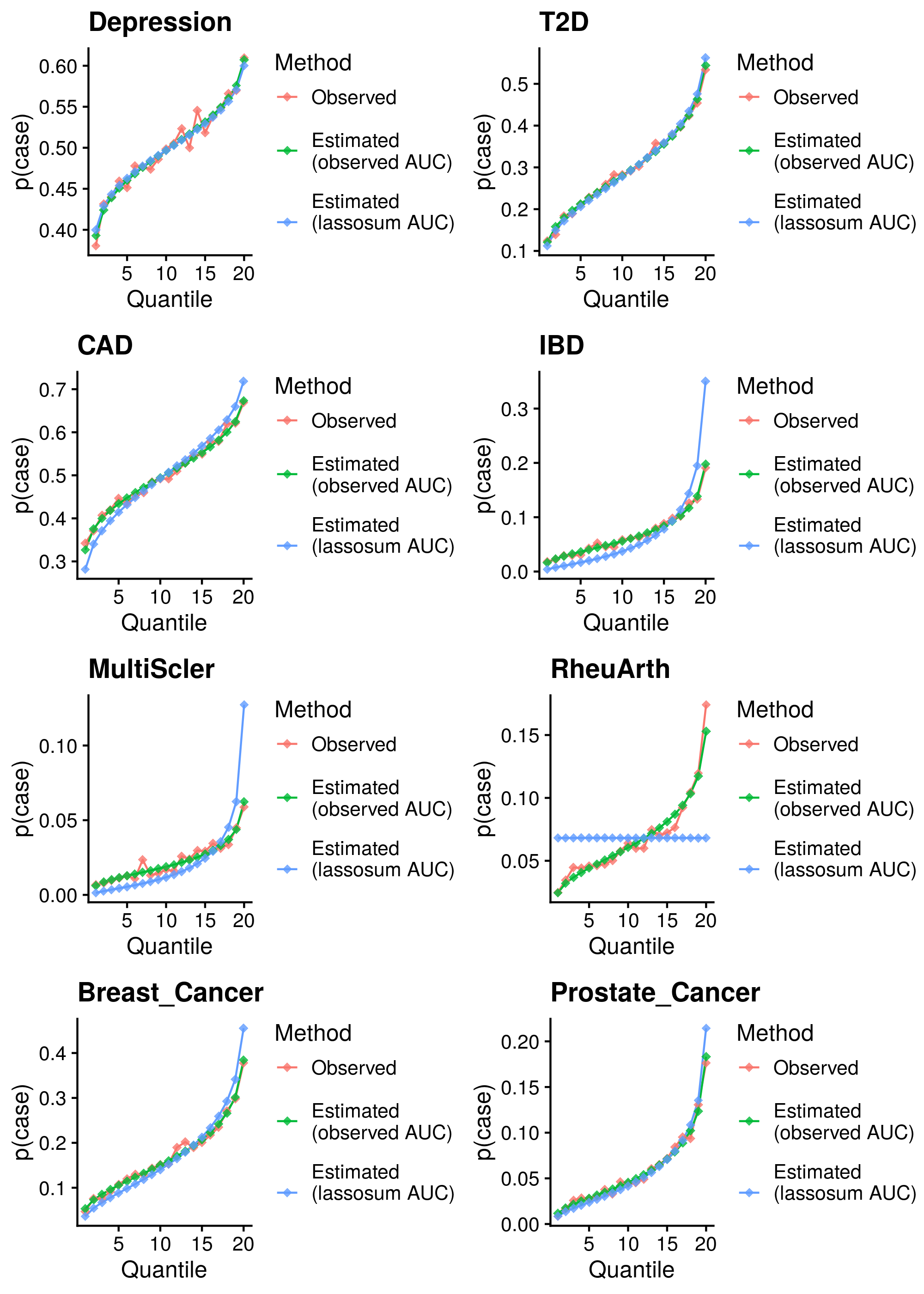
Phenotype	Correlation (95%CI)	Mean Abs. Diff.	N	Ncas	Ncon
Depression	0.985 (0.961-0.994)	1.6%	49999	24999	25000
T2D	0.996 (0.991-0.999)	3.4%	49999	14888	35111
CAD	0.995 (0.986-0.998)	4.3%	49999	25000	24999
IBD	0.963 (0.907-0.985)	38.6%	49999	3461	46538
MultiScler	0.915 (0.794-0.966)	43.7%	49999	1137	48862
RheuArth	-0.008 (-0.449-0.436)	40%	49999	3408	46591
Breast_Cancer	0.991 (0.978-0.997)	12.5%	49999	8512	41487
Prostate_Cancer	0.99 (0.976-0.996)	11.1%	50000	2927	47073

Median Cor. = 0.9875522; Mean Cor. = 0.8534752; Min. Cor. = -0.007714644; Max. Cor. = 0.9964987

Excluding RheuArth: Median Cor. = 0.9904925; Mean Cor. = 0.9765024; Min. Cor. = 0.9150213; Max. Cor. = 0.9964987

---

2.1.5.2 Continuous

Show code

library(data.table)
library(e1071)

source('/users/k1806347/brc_scratch/Software/MyGit/GenoPred/config_used/Target_scoring.config')

gwas<-c('COLL01','HEIG03','BODY04')
pheno<-c('Intelligence','Height','BMI')

n_quant<-20

files<-data.frame(pheno,gwas)

# Create function
mean_sd_quant.f <- function(PRS_R2=0.641, Outcome_mean=1, Outcome_sd=1, n_quantile=20){
  ### PRS quantiles with a continuous phenotype (Y)
  library(tmvtnorm)
  ###
  E_PRS = 0
  SD_PRS = sqrt(1)
  E_phenotype = Outcome_mean
  SD_phenotype = Outcome_sd 

  by_quant<-1/(n_quantile)
  PRS_quantile_bounds <- qnorm(p=seq(0, 1, by=by_quant), mean= E_PRS, sd= SD_PRS)
  lower_PRS_vec <- PRS_quantile_bounds[1:n_quantile]
  upper_PRS_vec <- PRS_quantile_bounds[2:(n_quantile+1)]
  
  mean_vec <- c(E_phenotype, E_PRS)
  sigma_mat <- matrix(sqrt(PRS_R2)*SD_phenotype*SD_PRS, nrow=2, ncol=2)
  sigma_mat[1,1] <- SD_phenotype^2
  sigma_mat[2,2] <- SD_PRS^2
  
  ### mean of phenotype within the truncated PRS distribution
  out_mean_Y <- rep(0, 20)
  ### SD of phenotype within the truncated PRS distribution
  out_SD_Y <- rep(0, 20)
  ### cov of Y and PRS given truncation on PRS
  out_cov_Y_PRS <- rep(0, 20)
  ### SD of PRS given truncation on PRS
  out_SD_PRS <- rep(0, 20)
  ### mean PRS given truncation on PRS
  out_mean_PRS <- rep(0, 20)
  
  for(i in 1:n_quantile){
    distribution_i <- mtmvnorm(mean = mean_vec,
        sigma = sigma_mat,
        lower = c(-Inf, lower_PRS_vec[i]),
        upper = c(Inf, upper_PRS_vec[i]),
        doComputeVariance=TRUE,
        pmvnorm.algorithm=GenzBretz())
        out_mean_Y[i] <- distribution_i$tmean[1]
        out_mean_PRS[i] <- distribution_i$tmean[2]
        out_SD_Y[i] <- sqrt(distribution_i$tvar[1,1])
        out_SD_PRS[i] <- sqrt(distribution_i$tvar[2,2])
        out_cov_Y_PRS[i] <- distribution_i$tvar[1,2]
  }
  
  out<-data.frame(q=1:n_quantile,
             q_min=lower_PRS_vec,
             q_max=upper_PRS_vec,
             x_mean=out_mean_Y,
             x_sd=out_SD_Y)
  
  return(out)

  out_mean_Y
  out_SD_Y
  
  out_mean_PRS
  out_SD_PRS
  out_cov_Y_PRS
}

# Read in lassosum R2
lassosum_R2<-read.csv('/scratch/users/k1806347/Analyses/AbsoluteRisk/Estimated_AUC_R2/lassosum/lassosum_R2.csv')

# Run analysis for each phenotype
res_all<-NULL
plots_all<-list()
cor_res<-NULL

for(i in 1:dim(files)[1]){
  # Read in pheno and prs data, and merge
  pheno_i<-fread(paste0(UKBB_output,'/Phenotype/PRS_comp_subset/UKBB.',files$pheno[i],'.txt'))
  names(pheno_i)[3]<-'pheno'
  prs_i<-fread(paste0(UKBB_output,'/PRS_for_interpretation/1KG_ref/DBSLMM/',files$gwas[i],'/UKBB.subset.w_hm3.',files$gwas[i],'.DBSLMM_profiles'))
  prs_i<-prs_i[,c('FID','IID',paste0(files$gwas[i], '_DBSLMM')), with=F]
  names(prs_i)[3]<-'prs'

  pheno_prs<-merge(pheno_i, prs_i, by=c('FID','IID'))
  
  # Read in AUC for PRS
  assoc<-fread(paste0('/scratch/users/k1806347/Analyses/AbsoluteRisk/Measured_AUC_R2/',files$pheno[i],'/UKBB.w_hm3.',files$gwas[i],'.EUR-PRSs.AllMethodComp.assoc.txt'))
  prs_r2<-assoc[grepl('DBSLMM', assoc$Predictor),]$Obs_R2
  
  # Assign individuals to observed PRS quantiles
  obs_quant<-quantile(pheno_prs$prs, prob = seq(0, 1, length = n_quant+1))
  pheno_prs$obs_quant<-as.numeric(cut( pheno_prs$prs, obs_quant, include.lowest = T))

  # Calculate mean and SD of each quantile that are cases
  obs_dist<-NULL
  for(k in 1:n_quant){
    obs_dist<-rbind(obs_dist, data.frame(Phenotype=files$pheno[i],
                                     Type='Observed',
                                     Quantile=k,
                                     q_min=obs_quant[k],
                                     q_max=obs_quant[k+1],
                                     x_mean=mean(pheno_prs$pheno[pheno_prs$obs_quant == k]),
                                     x_sd=sd(pheno_prs$pheno[pheno_prs$obs_quant == k])))
  }
  
  # Assign individuals to estimated PRS quantiles
  est_dist<-mean_sd_quant.f(PRS_R2 = prs_r2, Outcome_mean=mean(pheno_prs$pheno), Outcome_sd=sd(pheno_prs$pheno), n_quantile = n_quant)
  est_dist$q<-NULL
  est_dist<-data.frame(Phenotype=files$pheno[i],Type='\nEstimated\n(Observed R2)\n',Quantile=1:n_quant, est_dist)
  est_quant<-sort(unique(c(est_dist$q_min, est_dist$q_max)))
  pheno_prs$est_quant<-as.numeric(cut( pheno_prs$prs, est_quant, include.lowest = T))

  # Assign individuals to lassosum estimated PRS quantiles
  lasso_est_dist<-mean_sd_quant.f(PRS_R2 = lassosum_R2$lasso_R2[lassosum_R2$Phenotype == files$pheno[i]], Outcome_mean=mean(pheno_prs$pheno), Outcome_sd=sd(pheno_prs$pheno), n_quantile = n_quant)
  lasso_est_dist$q<-NULL
  lasso_est_dist<-data.frame(Phenotype=files$pheno[i],Type="Estimated\n(lassosum R2)\n",Quantile=1:n_quant, lasso_est_dist)
  lasso_est_quant<-sort(unique(c(lasso_est_dist$q_min, lasso_est_dist$q_max)))
  pheno_prs$lasso_est_quant<-as.numeric(cut( pheno_prs$prs, lasso_est_quant, include.lowest = T))
  
  quant_comp<-do.call(rbind, list(obs_dist, est_dist, lasso_est_dist))
  
  tmp<-cor.test(obs_dist$x_mean, est_dist$x_mean)
  tmp2<-cor.test(obs_dist$x_mean, lasso_est_dist$x_mean)
  
  cor_res<-rbind(cor_res,data.frame(Phenotype=files$pheno[i],
                                    Cor_mean=tmp$estimate,
                                    Cor_mean_Low95CI=tmp$conf.int[1],
                                    Cor_mean_High95CI=tmp$conf.int[2],
                                    Mean_perc_diff_mean=mean(abs(est_dist$x_mean-obs_dist$x_mean)/obs_dist$x_mean),
                                      Mean_perc_diff_sd=mean(abs(est_dist$x_sd-obs_dist$x_sd)/obs_dist$x_sd),
                                    Cor_mean_lasso=tmp2$estimate,
                                    Cor_mean_Low95CI_lasso=tmp2$conf.int[1],
                                    Cor_mean_High95CI_lasso=tmp2$conf.int[2],
                                    Mean_perc_diff_mean_lasso=mean(abs(lasso_est_dist$x_mean-obs_dist$x_mean)/obs_dist$x_mean),
                                      Mean_perc_diff_sd_lasso=mean(abs(lasso_est_dist$x_sd-obs_dist$x_sd)/obs_dist$x_sd),
                                    N=length(pheno_prs$pheno),
                                    Skewness=skewness(pheno_prs$pheno)))

  res_all<-rbind(res_all, quant_comp)
  
  library(ggplot2)
  library(cowplot)
  
  plots_all[[i]]<-ggplot(quant_comp, aes(x=Quantile, y=x_mean, colour=Type)) +
    geom_point(stat="identity", position=position_dodge(.5), alpha=0.8, shape=18, size=2) +
    geom_errorbar(aes(ymin=x_mean-x_sd, ymax=x_mean+x_sd), width=.2, position=position_dodge(.5), alpha=0.8) +
    labs(y="Mean (SD)", title=files$pheno[i], colour='Method') +
    theme_cowplot(12)

}

png(paste0('/scratch/users/k1806347/Analyses/AbsoluteRisk/Measured_AUC_R2/Mean_SD_Comp_lasso.png'), units='px', res=300, width=1750, height=2000)
  plot_grid(plotlist=plots_all, ncol = 1)
dev.off()

write.csv(cor_res, '/scratch/users/k1806347/Analyses/AbsoluteRisk/Measured_AUC_R2/Mean_SD_Comp_lasso.csv', row.names=F, quote=F)

Show results

Correlation between observed and estimated mean and standar deviation of outcome within polygenic score quantiles

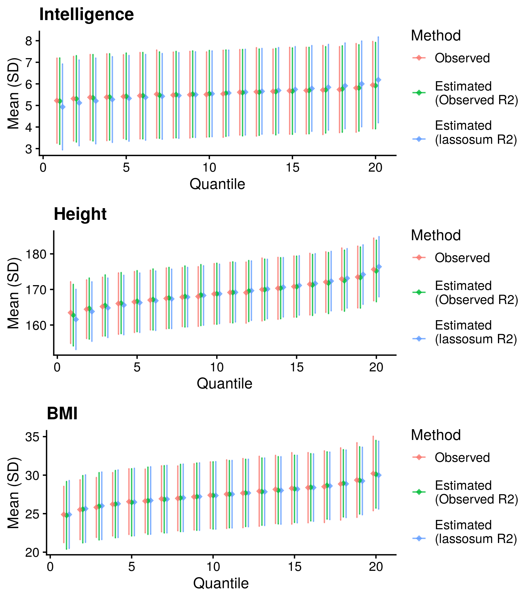
Phenotype	Correlation (95%CI)	Mean Abs. Diff. of Mean	Mean Abs. Diff. of SD	N	Skewness
Intelligence	0.992 (0.979-0.997)	1.9%	1.5%	50000	0.144
Height	0.996 (0.989-0.998)	0.2%	2.5%	49999	0.117
BMI	0.998 (0.995-0.999)	0.3%	6%	49999	0.592

Median Cor. of means = 0.9958381; Mean Cor. of means = 0.9952452; Min. Cor. of means = 0.9917264; Max. Cor. of means = 0.9981713

## Warning in mean.default(res$PercDiff_sd_mean_lasso): argument is not numeric or
## logical: returning NA

## Warning in min(res$PercDiff_sd_mean_lasso): no non-missing arguments to min;
## returning Inf

## Warning in max(res$PercDiff_sd_mean_lasso): no non-missing arguments to max;
## returning -Inf

Median mean %diff of SD = ; Mean mean %diff of SD = NA; Min. mean %diff of SD = Inf; Max. mean %diff of SD = -Inf

---

3 Prepare input for Impute.Me module

I need to download GWAS sumstats in an automated way, estimate the underlying heritability and produce reference standardised score files. GWAS sumstats will be downloaded from the GWAS catalogue.

3.1 Download GWAS sumstats

Show results

# Download latest GWAS catalogue index (22/11/2020)
# https://www.ebi.ac.uk/gwas/downloads/summary-statistics

# Read in the csv
gwas_list<-read.csv('~/brc_scratch/Data/GWAS_sumstats/GWAS_catalog/list_gwas_summary_statistics_22_Nov_2020.csv')

# Create a list GWAS catalogue IDs
gwas_ids<-c('GCST006901','GCST006900','GCST003045','GCST004773','GCST004296','GCST006572')
gwas_list_subset<-gwas_list[(gwas_list$Study.accession %in% gwas_ids),]

# List ftp downloads page
system(paste0('wget ftp://ftp.ebi.ac.uk/pub/databases/gwas/summary_statistics/  -P ~/brc_scratch/Data/GWAS_sumstats/GWAS_catalog/'))
ftp_list<-read.table('~/brc_scratch/Data/GWAS_sumstats/GWAS_catalog/index.html', sep='&', header=F)$V1
ftp_list<-ftp_list[grepl(paste(gwas_list_subset$Study.accession, collapse='|'), ftp_list)]
ftp_list<-gsub('>.*','',gsub('.*href=','',ftp_list))

# Download these summary statistics
for(gwas_i in ftp_list){
  system(paste0('wget ',gwas_i,' -O ~/brc_scratch/Data/GWAS_sumstats/GWAS_catalog/temp.txt'))
  temp_list<-read.table('~/brc_scratch/Data/GWAS_sumstats/GWAS_catalog/temp.txt', sep='&', header=F)$V1
  temp_list<-temp_list[grepl('href', temp_list)]
  temp_list<-gsub('>.*','',gsub('.*href=','',temp_list))
  if(sum(grepl('harmonised', temp_list) == T) > 0){
      system(paste0('wget -r ',gwas_i,'harmonised/ -P ~/brc_scratch/Data/GWAS_sumstats/GWAS_catalog/'))
  } else {
      system(paste0('wget -r ',gwas_i,' -P ~/brc_scratch/Data/GWAS_sumstats/GWAS_catalog/'))
  }
}

# After looking through the results for these studies, they are often not full summary statistics. Some are not in harmonised format, and some contain trans ancestry data. I think using the KCL repository might be a better option.