Defining ancestry in UKB
This page shows how individuals in UKB are assigned to the five 1KG Phase 3 super populations. The main analysis is performed using the ancesty_identfier.R script.
1 Format reference super population data
Show code
# Create an output file
system('mkdir -p /scratch/groups/ukbiobank/usr/ollie_pain/ReQC/defining_ancestry')

# Create a list of super population keep files
keep_list<-data.frame(Name=gsub('_.*','',list.files('/scratch/groups/biomarkers-brc-mh/Reference_data/1KG_Phase3/PLINK/super_pop_keep_files')),
                      File=paste0('/scratch/groups/biomarkers-brc-mh/Reference_data/1KG_Phase3/PLINK/super_pop_keep_files/',list.files('/scratch/groups/biomarkers-brc-mh/Reference_data/1KG_Phase3/PLINK/super_pop_keep_files')))
write.table(keep_list, '/scratch/groups/ukbiobank/usr/ollie_pain/ReQC/defining_ancestry/ref_super_pop_keep_list.txt', col.names=F, row.names=F, quote=F)

# Format .psam reference file for ancestry identifier
library(data.table)
psam<-fread('/scratch/groups/biomarkers-brc-mh/Reference_data/1KG_Phase3/PLINK/all_phase3.psam')
names(psam)[1]<-'sample'
psam<-psam[,c('sample','Population','SuperPop'),with=F]
names(psam)<-c('sample','pop','super_pop')
write.table(psam, '/scratch/groups/ukbiobank/usr/ollie_pain/ReQC/defining_ancestry/ref_pop_dat.txt', col.names = T, row.names = F, quote = F)
2 Create a fake fam file
Show code
library(data.table)

# Check number of individuals in genetic data
real_fam<-fread('/scratch/datasets/ukbiobank/ukb18177/genotyped/ukb18177_cal_chr1_v2_s488264.fam')

# Create a fam file with row number based IDs
fake_fam<-data.table(matrix(nrow = dim(real_fam)[1], ncol = 1))
fake_fam$V1<-1:dim(fake_fam)[1]
fake_fam$V2<-1:dim(fake_fam)[1]
fake_fam$V3<-0
fake_fam$V4<-0
fake_fam$V5<-0
fake_fam$V6<-0

fwrite(fake_fam, '/scratch/groups/ukbiobank/usr/ollie_pain/ReQC/fake_fam.fam', col.names = F, row.names = F, quote = F, sep=' ')
3 Defining ancestry
Assign to populations
sbatch -p brc,shared --mem=15G /users/k1806347/brc_scratch/Software/Rscript_singularity.sh /users/k1806347/brc_scratch/Software/MyGit/GenoPred/Scripts/Ancestry_identifier/Ancestry_identifier.R \
  --target_plink /scratch/datasets/ukbiobank/June2017/Genotypes/ukb_binary_v2 \
  --ref_plink_chr /scratch/groups/biomarkers-brc-mh/Reference_data/1KG_Phase3/PLINK/all_phase3.chr \
  --target_fam /scratch/groups/ukbiobank/usr/ollie_pain/ReQC/fake_fam.fam \
  --n_pcs 6 \
  --maf 0.05 \
  --geno 0.02 \
  --hwe 1e-6 \
  --memory 15000 \
  --plink /users/k1806347/brc_scratch/Software/plink1.9.sh \
  --plink2 /users/k1806347/brc_scratch/Software/plink2 \
  --output /scratch/groups/ukbiobank/usr/ollie_pain/ReQC/defining_ancestry/UKBB.Ancestry \
  --ref_pop_scale /scratch/groups/ukbiobank/usr/ollie_pain/ReQC/defining_ancestry/ref_super_pop_keep_list.txt \
  --pop_data /scratch/groups/ukbiobank/usr/ollie_pain/ReQC/defining_ancestry/ref_pop_dat.txt \
  --prob_thresh 0.5
3.1 Describe results
The predictive utility, as estimated using 5-fold CV in the 1KG Phase 3 sample, is summarised in the file called UKBB.Ancestry.pop_model_prediction_details.txt.
Show files contents
## glmnet
##
## 2504 samples
##    6 predictor
##    5 classes: 'AFR', 'AMR', 'EAS', 'EUR', 'SAS'
##
## No pre-processing
## Resampling: Cross-Validated (5 fold)
## Summary of sample sizes: 2003, 2002, 2003, 2003, 2005
## Resampling results across tuning parameters:
##
##   alpha  lambda        logLoss     AUC        prAUC      Accuracy   Kappa
##   0.10   0.0007804186  0.02268761  0.9999013  0.9890034  0.9948096  0.9934457
##   0.10   0.0078041855  0.06796617  0.9995560  0.9881168  0.9920167  0.9899164
##   0.10   0.0780418555  0.28459560  0.9995973  0.9877190  0.9820367  0.9772926
##   0.55   0.0007804186  0.02047993  0.9998982  0.9890189  0.9952104  0.9939517
##   0.55   0.0078041855  0.06413937  0.9995518  0.9881142  0.9920167  0.9899164
##   0.55   0.0780418555  0.32782661  0.9996558  0.9877274  0.9676606  0.9590715
##   1.00   0.0007804186  0.01508929  0.9999457  0.9893087  0.9964072  0.9954632
##   1.00   0.0078041855  0.05384136  0.9996831  0.9885685  0.9928135  0.9909239
##   1.00   0.0780418555  0.36186034  0.9993721  0.9869401  0.9544781  0.9423275
##   Mean_F1    Mean_Sensitivity  Mean_Specificity  Mean_Pos_Pred_Value
##   0.9939270  0.9933352         0.9986971         0.9946299
##   0.9904634  0.9893269         0.9979981         0.9920118
##   0.9778507  0.9749418         0.9955008         0.9829529
##   0.9944160  0.9939149         0.9987976         0.9950304
##   0.9904634  0.9893269         0.9979981         0.9920118
##   0.9589684  0.9541634         0.9918943         0.9712239
##   0.9958388  0.9953691         0.9990899         0.9963778
##   0.9914607  0.9904698         0.9981976         0.9927176
##   0.9407505  0.9351406         0.9885769         0.9613764
##   Mean_Neg_Pred_Value  Mean_Precision  Mean_Recall  Mean_Detection_Rate
##   0.9987520            0.9946299       0.9933352    0.1989619
##   0.9981140            0.9920118       0.9893269    0.1984033
##   0.9958604            0.9829529       0.9749418    0.1964073
##   0.9988450            0.9950304       0.9939149    0.1990421
##   0.9981140            0.9920118       0.9893269    0.1984033
##   0.9926990            0.9712239       0.9541634    0.1935321
##   0.9991369            0.9963778       0.9953691    0.1992814
##   0.9982941            0.9927176       0.9904698    0.1985627
##   0.9898817            0.9613764       0.9351406    0.1908956
##   Mean_Balanced_Accuracy
##   0.9960161
##   0.9936625
##   0.9852213
##   0.9963563
##   0.9936625
##   0.9730288
##   0.9972295
##   0.9943337
##   0.9618587
##
## logLoss was used to select the optimal model using the smallest value.
## The final values used for the model were alpha = 1 and lambda = 0.0007804186.
##
## Confusion matrix without threshold:
##         pred AFR pred AMR pred EAS pred EUR pred SAS
## obs AFR      659        2        0        0        0
## obs AMR        3      340        0        4        0
## obs EAS        0        0      504        0        0
## obs EUR        0        0        0      503        0
## obs SAS        0        0        0        0      489
##
## Confusion matrix with 0.5 threshold:
##         pred AFR pred AMR pred EAS pred EUR pred SAS
## obs AFR      659        2        0        0        0
## obs AMR        3      340        0        4        0
## obs EAS        0        0      504        0        0
## obs EUR        0        0        0      503        0
## obs SAS        0        0        0        0      489
The accuracy of the mode in 1KG is very high, and the confusion matrix shows there were only a few incorrectly assigned individuals.
The script also create a plot showing the PCs of target sample participants compared to the reference populations.
Show plot
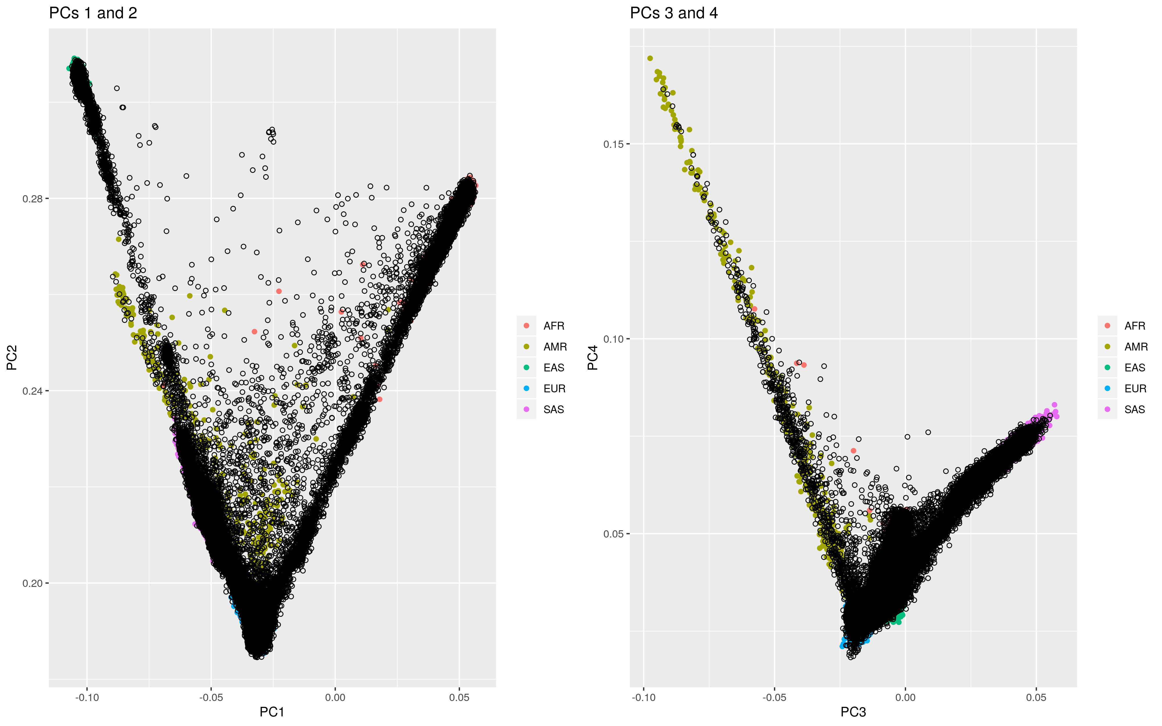
UKB PCs compared to 1KG populations
Show log file
## #################################################################
## # Ancestry_identifier.R
## # For questions contact Oliver Pain (oliver.pain@kcl.ac.uk)
## #################################################################
## Analysis started at 2021-01-26 14:15:20
## Options are:
## Options are:
## $target_plink_chr
## [1] NA
##
## $target_plink
## [1] "/scratch/datasets/ukbiobank/June2017/Genotypes/ukb_binary_v2"
##
## $ref_plink_chr
## [1] "/scratch/groups/biomarkers-brc-mh/Reference_data/1KG_Phase3/PLINK/all_phase3.chr"
##
## $target_fam
## [1] "/scratch/groups/ukbiobank/usr/ollie_pain/ReQC/fake_fam.fam"
##
## $maf
## [1] 0.05
##
## $geno
## [1] 0.02
##
## $hwe
## [1] 1e-06
##
## $n_pcs
## [1] 6
##
## $plink
## [1] "/users/k1806347/brc_scratch/Software/plink1.9.sh"
##
## $plink2
## [1] "/users/k1806347/brc_scratch/Software/plink2"
##
## $output
## [1] "/scratch/groups/ukbiobank/usr/ollie_pain/ReQC/defining_ancestry/UKBB.Ancestry"
##
## $ref_pop_scale
## [1] "/scratch/groups/ukbiobank/usr/ollie_pain/ReQC/defining_ancestry/ref_super_pop_keep_list.txt"
##
## $pop_data
## [1] "/scratch/groups/ukbiobank/usr/ollie_pain/ReQC/defining_ancestry/ref_pop_dat.txt"
##
## $model_method
## [1] "glmnet"
##
## $SD_rule
## [1] FALSE
##
## $prob_thresh
## [1] 0.5
##
## $memory
## [1] 15000
##
## $help
## [1] FALSE
##
## $output_dir
## [1] "/scratch/groups/ukbiobank/usr/ollie_pain/ReQC/defining_ancestry/"
##
## Analysis started at 2021-01-26 14:15:20
## Merging per chromosome reference data...Done!
## Identifying LD independent SNPs based on reference data...Done!
## Computing reference PCs...Done!
## Deriving model predicting ref_pop groups...Done!
## Calculating PCs in the target sample...Done!
## Plotting target sample PCs on reference...Done!
## Estimating probability of each population...Done!
## ----------
## N per group based on model:
##   Group      N
## 1   AFR   9127
## 2   AMR   2033
## 3   EAS   2654
## 4   EUR 463275
## 5   SAS  10569
## ----------
## ----------
## N per group based on 3SD rule:
##   Group      N
## 1   AFR   7698
## 2   AMR 467268
## 3   EAS   1895
## 4   EUR 456861
## 5   SAS   8467
## ----------
## Analysis finished at 2021-01-26 15:18:46
## Analysis duration was 1.06 hours
The log file shows the number of individuals within each super population based on the elastic net mode and the 3 standard deviation rule. You can see that the elastic net results vary most for the AMR super population due to the large degree of admixture in this super population leading to a high SD.
3.2 Show distribution of probabilities
Show code and figures
library(data.table)

probs<-fread('/scratch/groups/ukbiobank/usr/ollie_pain/ReQC/defining_ancestry/UKBB.Ancestry.model_pred')

probs_melt<-melt(probs[,-1:-2])
## Warning in melt.data.table(probs[, -1:-2]): id.vars and measure.vars are
## internally guessed when both are 'NULL'. All non-numeric/integer/logical type
## columns are considered id.vars, which in this case are columns []. Consider
## providing at least one of 'id' or 'measure' vars in future.library(ggplot2)
# Basic density
ggplot(probs_melt, aes(x=value, fill=variable)) +
geom_density(bw=0.01, alpha=0.5) +
labs(x='Probability')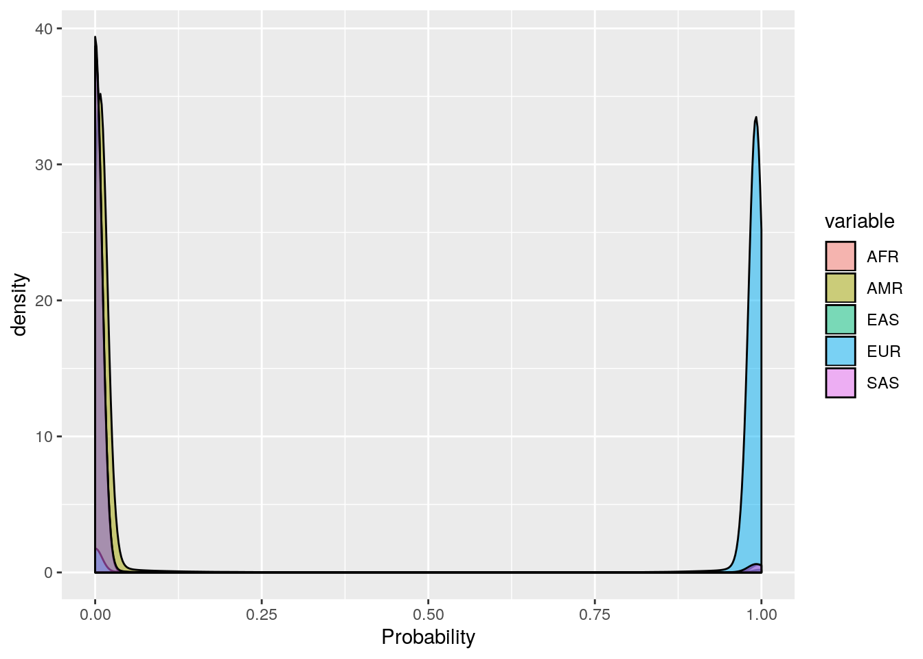
ggplot(probs_melt[probs_melt$value < 0.01,], aes(x=value, fill=variable)) +
  geom_density(bw=0.001, alpha=0.5) +
  labs(x='Probability')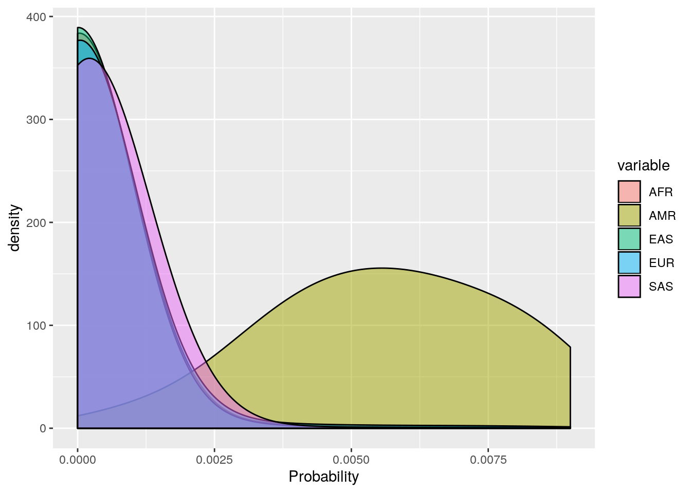
ggplot(probs_melt[probs_melt$value < 0.01,], aes(x=value, fill=variable)) +
  geom_density(bw=0.001, alpha=0.5) +
  geom_histogram(aes(y=..density..),binwidth=0.001, alpha=0.5) +
  labs(x='Probability')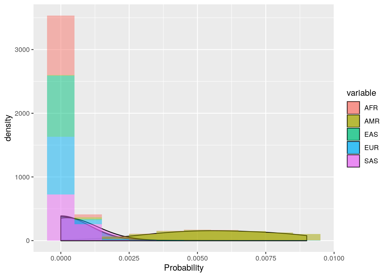
ggplot(probs_melt[probs_melt$value > 0.95,], aes(x=value, fill=variable)) +
  geom_density(bw=0.001, alpha=0.5) +
  labs(x='Probability')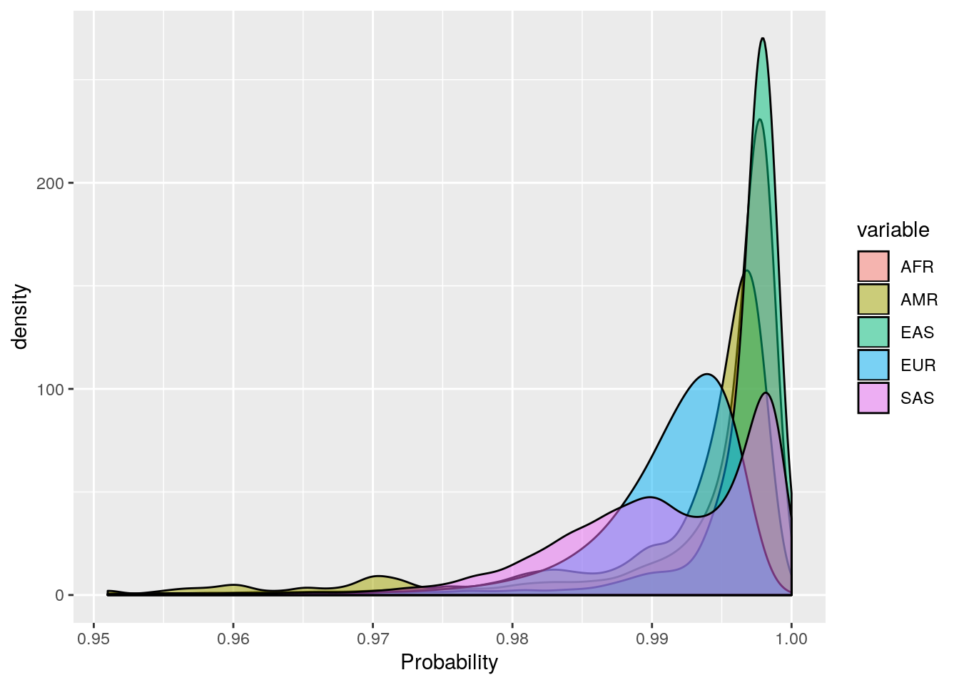
ggplot(probs_melt[probs_melt$value > 0.95,], aes(x=value, fill=variable)) +
  geom_density(bw=0.001, alpha=0.5) +
  geom_histogram(aes(y=..density..),binwidth=0.001, alpha=0.5) +
  labs(x='Probability')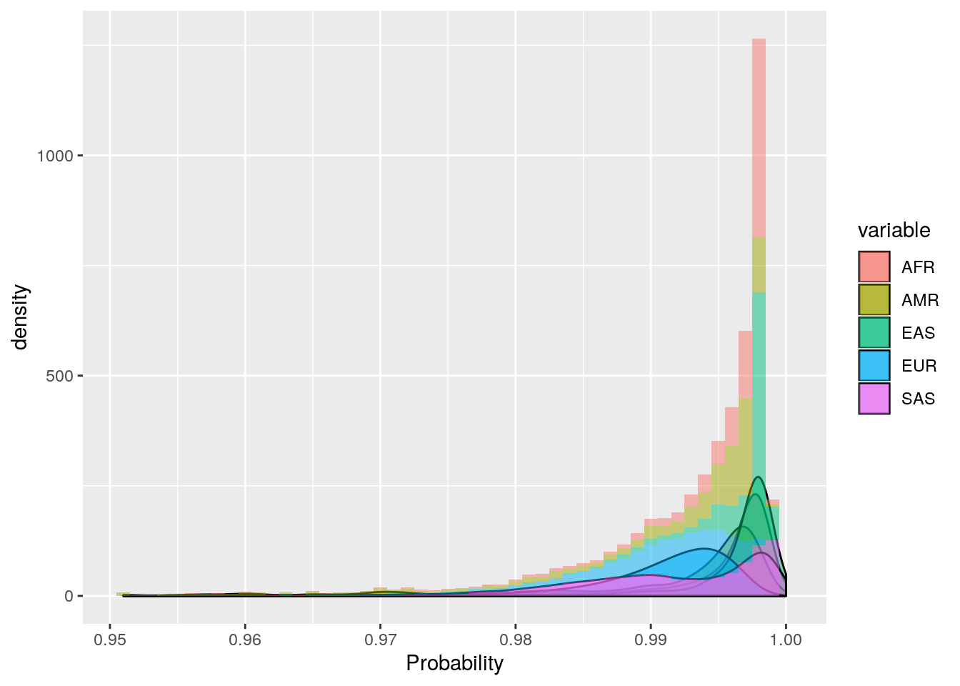
ggplot(probs_melt[probs_melt$value > 0.4 & probs_melt$value < 0.6,], aes(x=value, fill=variable)) +
  geom_density(bw=0.005, alpha=0.5) +
  labs(x='Probability')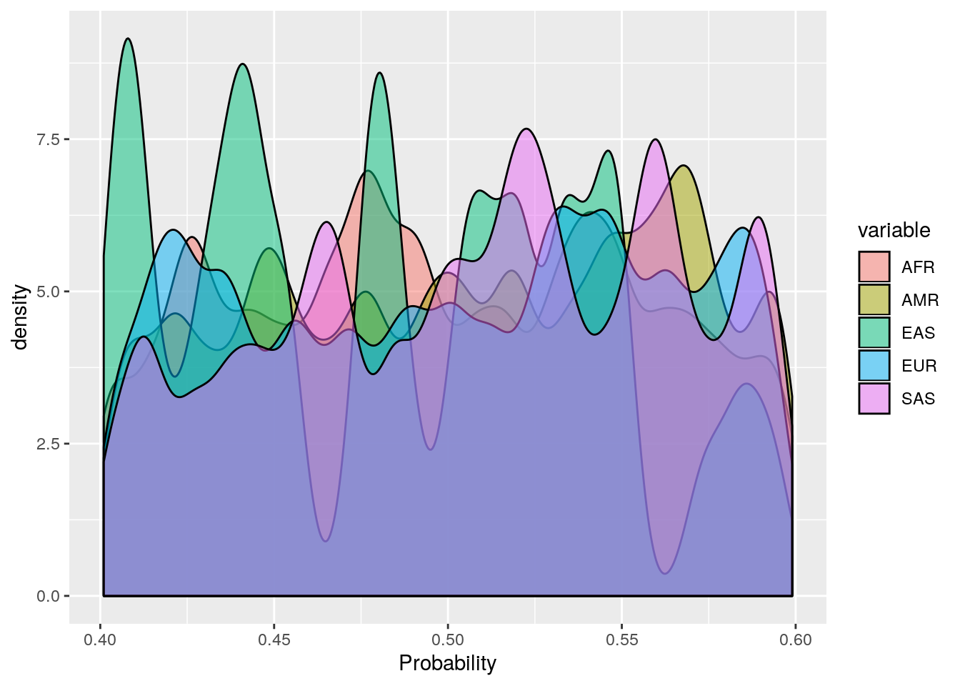
ggplot(probs_melt[probs_melt$value > 0.3 & probs_melt$value < 0.7,], aes(x=value, fill=variable)) +
  geom_density(bw=0.01, alpha=0.5) +
  geom_histogram(aes(y=..density..),binwidth=0.05, alpha=0.5) +
  labs(x='Probability')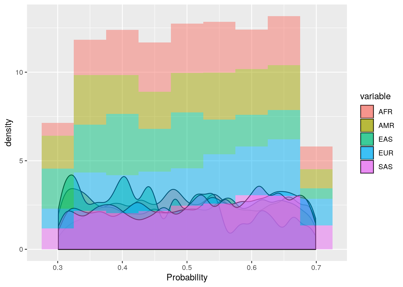
These plots show that the vast majority of individuals have a very high probability for one super population. The distribution of probabilities is less skewed (i.e. less certain) for the AMR super population, as we would predict due to a large degree of ad mixture. These results suggest that the probability threshold could be far more stringent without removing many individuals.
Show how many individuals would be present in each super population as the probability threshold changes.
Show code and results
library(data.table)

probs<-fread('/scratch/groups/ukbiobank/usr/ollie_pain/ReQC/defining_ancestry/UKBB.Ancestry.model_pred')

probs$max_prob<-apply(probs[,-1:-2], 1, max)

N_groups<-data.frame(pop=c('AFR','AMR','EAS','EUR','SAS'))
for(i in c(0,0.5,0.6,0.7,0.8,0.85,0.9,0.95)){
  probs_tmp<-probs[probs$max_prob > i,c('AFR','AMR','EAS','EUR','SAS')]
  tmp<-names(probs_tmp)[apply(probs_tmp,1,which.max)]

  N_groups$tmp<-NA
  for(j in c('AFR','AMR','EAS','EUR','SAS')){
    N_groups$tmp[N_groups$pop == j]<-sum(tmp == j)
  }

  names(N_groups)[names(N_groups) == 'tmp']<-paste0('N_',i)
}

print(N_groups)
## pop N_0 N_0.5 N_0.6 N_0.7 N_0.8 N_0.85 N_0.9 N_0.95
## 1 AFR 9287 9127 8946 8763 8437 8293 8221 8021
## 2 AMR 2214 2033 1563 1078 754 699 656 593
## 3 EAS 2675 2654 2624 2602 2576 2565 2549 2519
## 4 EUR 463495 463275 462882 462408 461753 461092 459670 456416
## 5 SAS 10706 10569 10378 10157 9920 9768 9573 9329This shows that using a more stringent probability theshold does not substantially reduce the number of individuals in each super population.